A Class of Models with the Potential to Represent Fundamental Physics
  1. Introduction
  2. Basic Form of Models
  3. Typical Behaviors
  4. Limiting Behavior and Emergent Geometry
  5. The Updating Process for String Substitution Systems
  6. The Updating Process in Our Models
  7. Equivalence and Computation in Our Models
  8. Potential Relation to Physics
  9. Additional Material
  10. References
  11. Index

2.9 Connectedness

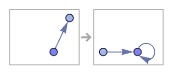
All the rules we have seen so far maintain connectedness. It is, however, straightforward to set up rules that do not. An obvious example is:

{{x, y}} -> {{y, y}, {x, z}}
RulePlot[ResourceFunction[ "WolframModel"][{{x, y}} -> {{x, z}, {y, y}}]]
Framed[#, FrameStyle -> LightGray] & /@ ResourceFunction[ "WolframModel"][{{x, y}} -> {{x, z}, {y, y}}, {{1, 2}}, 5, "StatesPlotsList"]

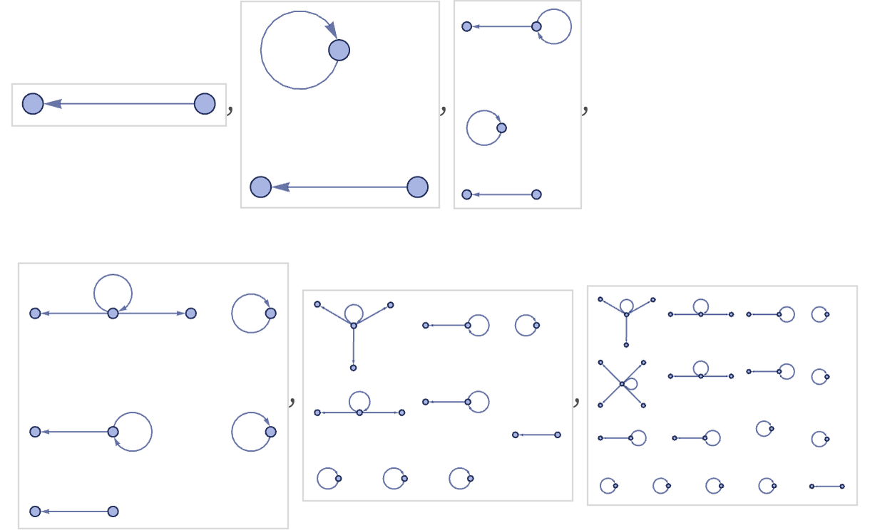
At step n, there are 2n+1 components altogether, with the largest component having n + 1 relations.

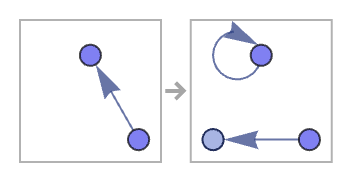
Rules that are themselves connected can produce disconnected results:

{{x, y}} -> {{x, x}, {z, x}}
RulePlot[ResourceFunction[ "WolframModel"][{{x, y}} -> {{x, x}, {z, x}}]]
Framed[#, FrameStyle -> LightGray] & /@ ResourceFunction[ "WolframModel"][{{x, y}} -> {{x, x}, {z, x}}, {{1, 2}}, 3, "StatesPlotsList"]

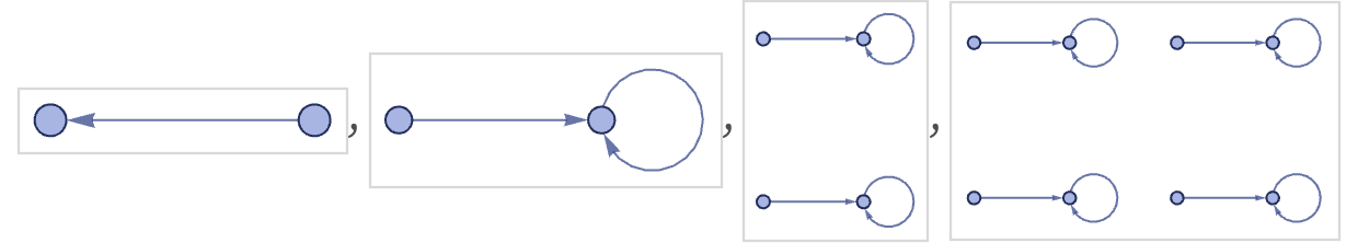
Rules whose left-hand sides are connected in a sense operate locally on hypergraphs. But rules with disconnected left-hand sides (such as {{x},{y}}{{x,y}}) can operate non-locally and in effect knit together elements from anywherethough such a process is almost inevitably rife with ambiguity.