A Class of Models with the Potential to Represent Fundamental Physics
  1. Introduction
  2. Basic Form of Models
  3. Typical Behaviors
  4. Limiting Behavior and Emergent Geometry
  5. The Updating Process for String Substitution Systems
  6. The Updating Process in Our Models
  7. Equivalence and Computation in Our Models
  8. Potential Relation to Physics
  9. Additional Material
  10. References
  11. Index

5.4 Typical Multiway Graph Structures

Before considering further features of the updating process, it is helpful to discuss the typical kinds of multiway graphs that are generated from string substitution systems. Much as for our primary models based on general relations (hypergraphs), we can assign signatures to string substitution system rules based on the lengths of the strings in each transformation. For example, we will say that the rule {A BBB, BB A} has signature 2: 13, 21, where the initial 2 indicates the number of distinct possible elements (here A and B) that occur in the rule.

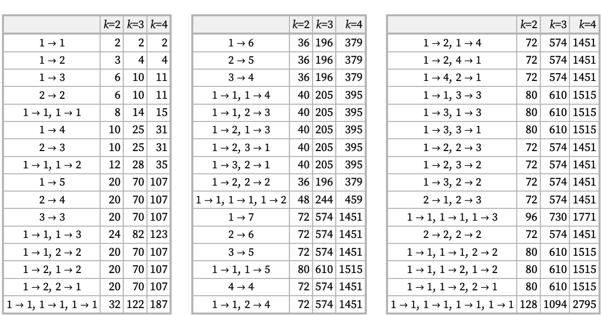
With a signature of the form k: n1n2, n3n4, there are nominally kni possible rules. However, many of these rules are equivalent under renaming of elements or reversal of strings. Taking this into account, the number of inequivalent possible rules for various cases is:

CloudGet["https://wolfr.am/LjVGUfk9"] Row[Grid[#, Alignment -> {{Center, Right, Right, Right}, Inherited}, Background -> {None, {GrayLevel[0.94], White}}, BaseStyle -> {"Text", Medium}, Dividers -> {Thread[{1, 5, 9, 13} -> Directive[Thick, GrayLevel[0.7]]], Thread[{1, 2, 18} -> Directive[Thick, GrayLevel[0.7]]]}, Frame -> All, FrameStyle -> GrayLevel[0.7], ItemSize -> {Automatic, Automatic}] & /@ (Prepend[#, (Style[#, FontSize -> .95 Inherited, FontFamily -> "Source Serif Pro"] & /@ Flatten[ Prepend[Table[ TraditionalForm[Row[{Style["k", Italic], "=", k}]], {k, 2, 4}], ""]])] & /@ Partition[ MapAt[Style[Row[#, ","], FontSize -> .95 Inherited] &, allres, {All, 1}], 16]), Spacer[10], BaselinePosition -> Top]

Rules with signature k: 1n must always be totally causal invariant. If they are started from strings of length 1, their states graphs can never branch. However, with strings of length more than 1, branching can (but may not) occur, as in this example of A AB started from three strings of length 2:

ResourceFunction["MultiwaySystem"][{"A" -> "AB"}, ResourceFunction["StringTuples"]["AB", 2], 4, "StatesGraph"]

With initial conditions AAA and AAAA, this rule produces the following states graphs:

{Graph[ResourceFunction["MultiwaySystem"][{"A" -> "AB"}, {#}, 5, "StatesGraphStructure"], ImageSize -> 100], Graph3D[ResourceFunction["MultiwaySystem"][{"A" -> "AB"}, {#}, 4, "StatesGraphStructure"], GraphLayout -> "SpringElectricalEmbedding", ImageSize -> 165, BaseStyle -> {Graphics3DBoxOptions -> {Method -> {"ShrinkWrap" -> True}}}, EdgeStyle -> Directive[Hue[0.62, 0.05, 0.55], Opacity[.6]]]} & /@ {"AAA", "AAAA"}

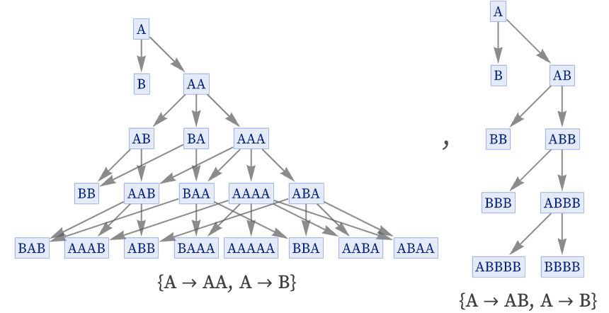
Even the rule A AA can produce states graphs like these if it has initial conditions that contain Bs as “separators”:

ResourceFunction[ "MultiwaySystem"][{"A" -> "AA"}, "ABA", 4, "StatesGraph"]

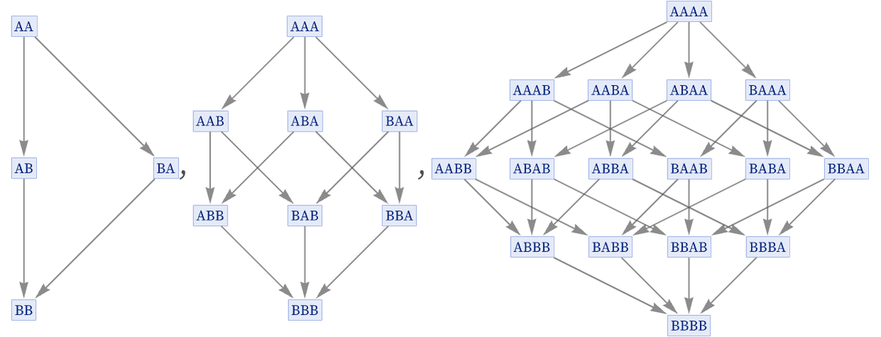
And as a seemingly even more trivial example, the rule A B with an initial condition containing n As gives a states graph corresponding to an n-dimensional cube (with a total of 2n nodes):

Table[ResourceFunction["MultiwaySystem"][{"A" -> "B"}, StringRepeat["A", n], 5, "StatesGraph"], {n, 2, 4}]

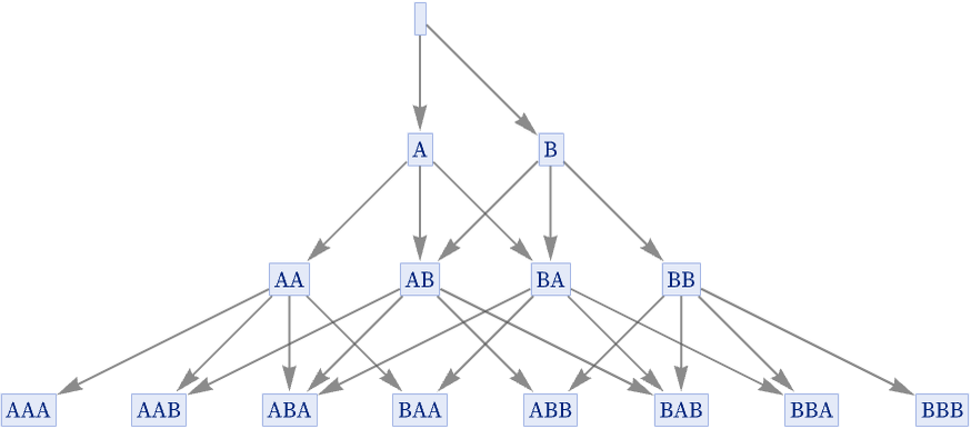
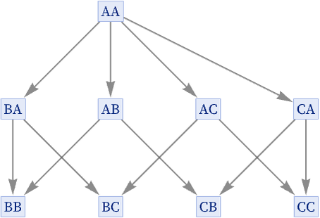
With multiple rules, one can get tree-like structures, with exponentially increasing numbers of states. The simplest case is the 2: 01, 01 rule { A, B} starting with the null string:

ResourceFunction["MultiwaySystem"][{"" -> "A", "" -> "B"}, "", 3, "EvolutionGraph"] // LayeredGraphPlot

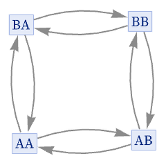
With multiple rules, even with single-symbol left-hand sides, causal invariance is no longer guaranteed. Of the 8 inequivalent 2: 11, 11 rules, all are totally causal invariant, although the rule {A B, B A} achieves this through cyclic behavior:

ResourceFunction["MultiwaySystem"][{"A" -> "B", "B" -> "A"}, ResourceFunction["StringTuples"]["AB", 2], 4, "StatesGraph"]

Among the 14 inequivalent 3: 11, 11 rules, all but two are totally causal invariant. The exceptions are the cyclic rule, and also the rule {A B, A C}, which in effect terminates before its B and C branches can reconverge:

ResourceFunction["MultiwaySystem"][{"A" -> "B", "A" -> "C"}, "AA", 4, "StatesGraph"]

The 12 inequivalent 2: 12, 11 rules yield the following states graphs when run for 4 steps starting from all possible length-3 strings of As and Bs:

UndirectedGraph[ ResourceFunction["MultiwaySystem"][#, ResourceFunction["StringTuples"]["AB", 3], 4, "StatesGraphStructure"], ImageSize -> 90, Frame -> True, FrameStyle -> LightGray] & /@ ResourceFunction["EnumerateSubstitutionSystemRules"][{1 -> 2, 1 -> 1}, 2]

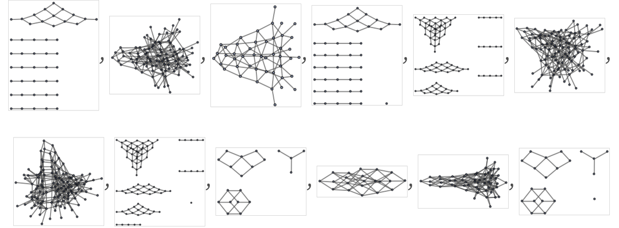
All but three of these rules are totally causal invariant. Among causal invariant ones are:

Labeled[ResourceFunction["MultiwaySystem"][#, "A", 4, "StatesGraph"], Text[#, BaseStyle -> {GrayLevel[.25], FontSize -> .9 Inherited, FontFamily -> "Source Serif Pro"}]] & /@ {{"A" -> "AB", "B" -> "A"}, {"A" -> "BB", "B" -> "A"}}

After more steps these yield:

{LayeredGraphPlot[ ResourceFunction["MultiwaySystem"][{"A" -> "AB", "B" -> "A"}, "A", 7, "StatesGraphStructure"], ImageSize -> {Automatic, 150}], Graph[ResourceFunction["MultiwaySystem"][{"A" -> "BB", "B" -> "A"}, "A", 9, "StatesGraphStructure"], ImageSize -> {Automatic, 150}]}

Examples of non-causal invariant 2: 12, 11 rules are:

Labeled[LayeredGraphPlot[ ResourceFunction["MultiwaySystem"][#[[1]], "A", 4, "StatesGraph"], #[[2]]], Text[#[[1]], BaseStyle -> {GrayLevel[.25], FontSize -> .9 Inherited, FontFamily -> "Source Serif Pro"}]] & /@ {{{"A" -> "AA", "A" -> "B"}, ImageSize -> 300}, {{"A" -> "AB", "A" -> "B"}, ImageSize -> 80}}

After more steps these yield:

{LayeredGraphPlot[ ResourceFunction["MultiwaySystem"][{"A" -> "AA", "A" -> "B"}, "A", 6, "StatesGraphStructure"], ImageSize -> {Automatic, 150}], Graph[ResourceFunction["MultiwaySystem"][{"A" -> "AB", "A" -> "B"}, "A", 11, "StatesGraphStructure"], ImageSize -> {Automatic, 150}]}

When we look at rules with larger signatures, the vast majority at least superficially show the same kinds of behavior that we have already seen.

Like for the hypergraphs from our models that we considered in previous sections, we can study the limiting structure of states graphs generated in multiway systems, and see what emergent geometry they may have. And in analogy to Vr(X) for hypergraphs, we can define a quantity Mt(S) which specifies the total number of distinct states reached in the multiway system after t steps of evolution starting from a state S.

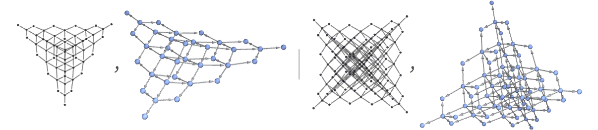
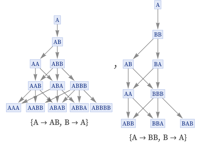
For the rule {A AB} mentioned above, the geometry of the multiway graph obtained by starting from n As is effectively a regular n-dimensional grid:

Graph[ResourceFunction["MultiwaySystem"][{"A" -> "AB"}, {"A"}, 5, "StatesGraph"], GraphLayout -> "SpringElectricalEmbedding"]
Graph[ResourceFunction["MultiwaySystem"][{"A" -> "AB"}, {"AA"}, 5, "StatesGraph"], GraphLayout -> "SpringElectricalEmbedding"]
Graph3D[ResourceFunction["MultiwaySystem"][{"A" -> "AB"}, {"AAA"}, 3, "StatesGraph"], GraphLayout -> "SpringEmbedding", EdgeStyle -> Directive[Hue[0.62, 0.05, 0.55], Opacity[.6]]]

Mt(An) in this case is then an n-fold nested sum of t 1s:

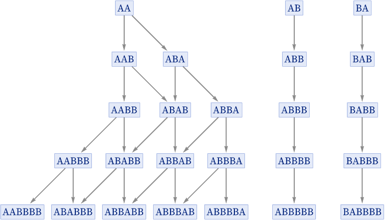
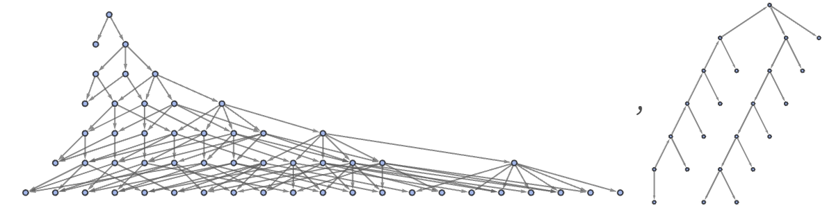
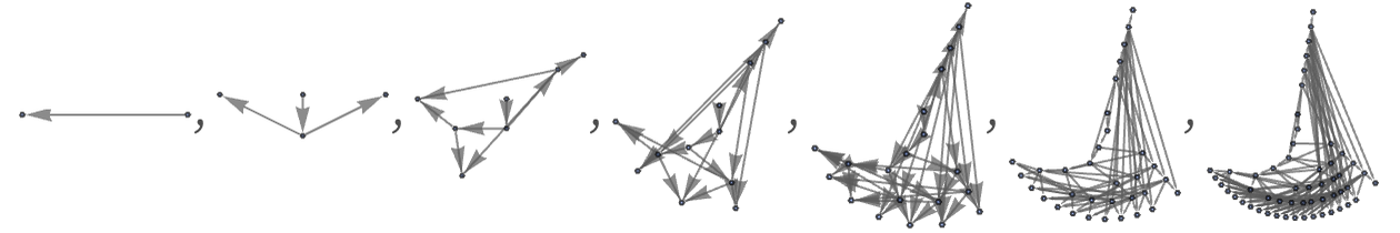
Some rules create states graphs that are trees, with Mt~mt. Other rules do not explicitly give trees, but still give exponentially increasing Mt. An example is {A AB, B A}, for which Mt is a sum of Fibonacci numbers, and successive states graphs can be rendered as:

Table[TreePlot[ ResourceFunction["MultiwaySystem"][{"A" -> "AB", "B" -> "A"}, "A", t, "StatesGraphStructure"], "A" -> Center, ImageSize -> 80], {t, 7}]

Note that rules with both polynomial and exponential growth in Mt can exhibit causal invariance.

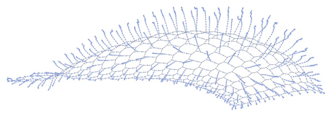
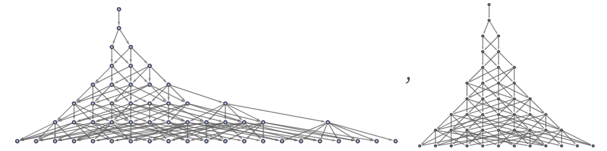
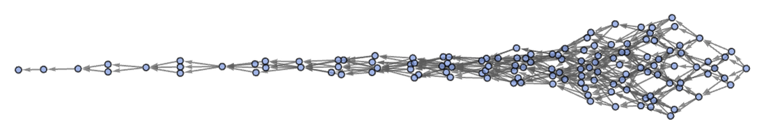
It is not uncommon to find rules with fairly long transients. A simple example is the totally causal invariant rule {A BBB, BBBB A}. When started from n As this stabilizes after 7n steps, with ~2.8n states, with a states graph like:

ResourceFunction["MultiwaySystem"][{"A" -> "BBB", "BBBB" -> "A"}, {"AAAA"}, 30, "StatesGraphStructure"]

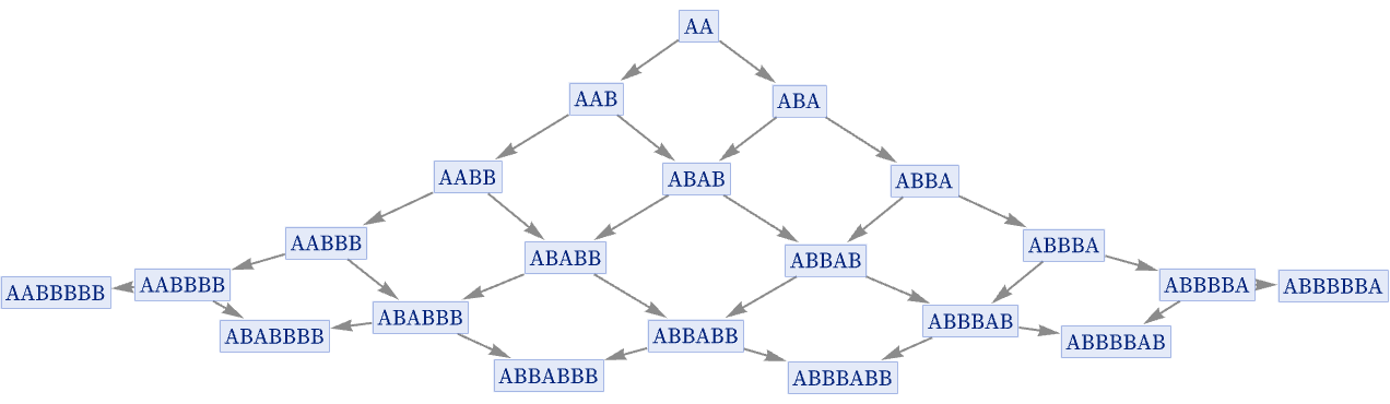
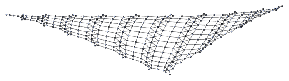
Rules typically seem to have either asymptotically exponential or asymptotically polynomial Mt. (This may have some analogy with what is seen in the growth of groups [57][58][22].) Among rules with polynomial growth, it is typical to see fairly regular grid-like structures. An example is the rule

{"AB" -> "A", "ABA" -> "BBAABB"}

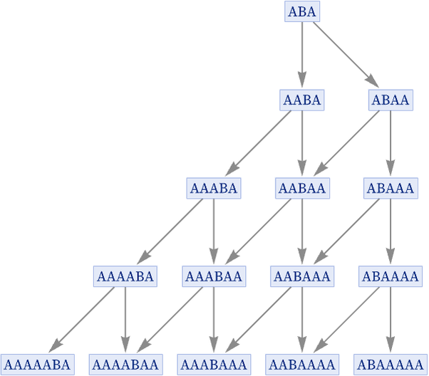
which from initial condition ABAA gives states graph:

ResourceFunction["MultiwaySystem"][{"AB" -> "A", "ABA" -> "BBAABB"}, {"ABAA"}, 40, "StatesGraphStructure"]

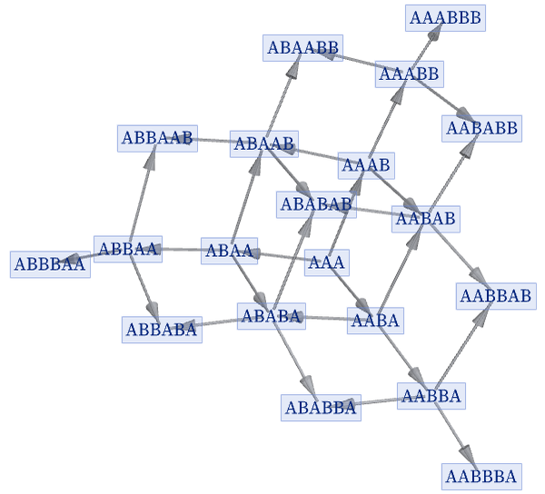
With the slightly different initial condition ABAAA, the states graph has a more elaborate structure

ResourceFunction["MultiwaySystem"][{"AB" -> "A", "ABA" -> "BBAABB"}, {"ABAAA"}, 25, "StatesGraphStructure"]

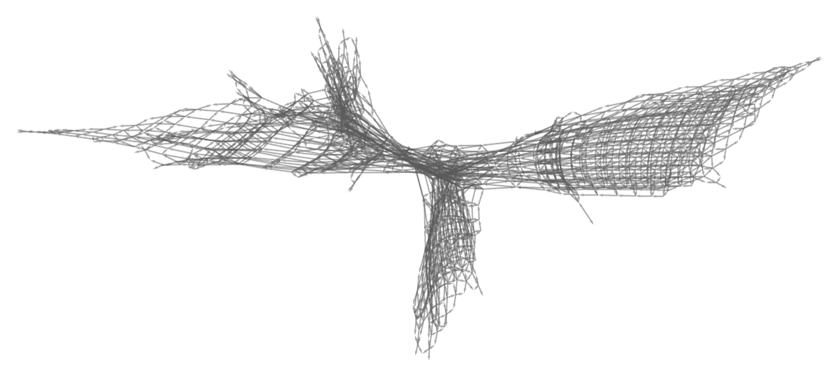
and the form of Mt is more complicated (though ~t2 and ultimately quasiperiodic); the second differences of Mt in this case are:

MultiwayGrowthList[rule_, init_List, t_, max_Integer] := Catch[Last /@ NestList[ Function[ s, {Join[First[s], #], #} &[ If[Length[#] > max, Throw[None], #] &@ Complement[Union[Flatten[StringReplaceList[Last[s], rule]]], First[s]]]], {{}, init}, t]]; ListLinePlot[ Differences[ Length /@ MultiwayGrowthList[{"AB" -> "A", "ABA" -> "BBAABB"}, {"ABAAA"}, 100, 4000], 2], Frame -> True, PlotStyle -> ResourceFunction["WolframPhysicsProjectStyleData"][ "GenericLinePlot", "PlotStyles"]]

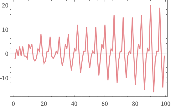
Another example of a somewhat complex structure occurs in the rule

{"ABA" -> "BBAA", "BAA" -> "AAB"}

that was discussed in [1:p205]. Starting from BABBAAB it gives the states graph:

ResourceFunction["MultiwaySystem"][{"ABA" -> "BBAA", "BAA" -> "AAB"}, {"BABBAAB"}, 100, "StatesGraphStructure", VertexSize -> 15]