A Class of Models with the Potential to Represent Fundamental Physics
  1. Introduction
  2. Basic Form of Models
  3. Typical Behaviors
  4. Limiting Behavior and Emergent Geometry
  5. The Updating Process for String Substitution Systems
  6. The Updating Process in Our Models
  7. Equivalence and Computation in Our Models
  8. Potential Relation to Physics
  9. Additional Material
  10. References
  11. Index

2.4 Self-Loops

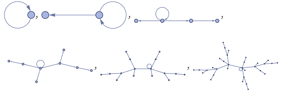
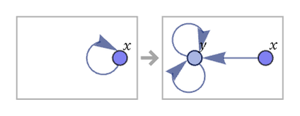
A relation can contain two identical elements, as in {0,0}, corresponding to a self-loop in a graph. Starting our first rule from a single self-loop, the self-loop effectively just stays marking the original node:

ResourceFunction[ "WolframModel"][{{{x, y}} -> {{x, y}, {y, z}}}, {{0, 0}}, 5]["StatesPlotsList", "MaxImageSize" -> 180]

However, with for example the rule:

{{x, y}} -> {{y, z}, {z, x}}
RulePlot[ResourceFunction[ "WolframModel"][{{x, y}} -> {{y, z}, {z, x}}], VertexLabels -> Automatic, "RulePartsAspectRatio" -> 0.25]

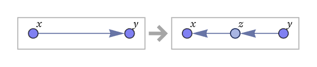
the self-loop effectively “takes over” the system, “inflating” to a 2n gon:

ResourceFunction["WolframModelPlot"][#, "MaxImageSize" -> 100] & /@ ResourceFunction[ "WolframModel"][{{x, y}} -> {{y, z}, {z, x}}, {{1, 1}}, 5, "StatesList"]

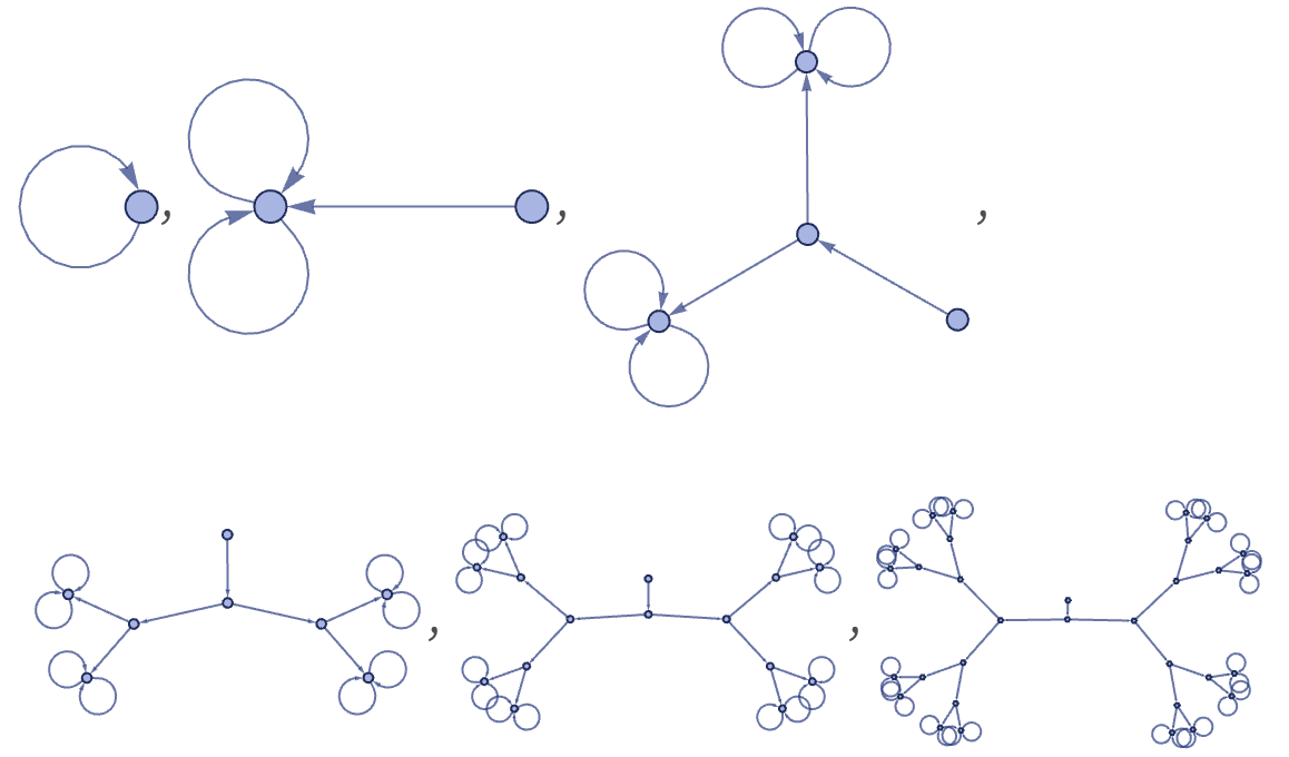
The rule can also contain self-loops. An example is

{{x, x}} -> {{y, y}, {y, y}, {x, y}}

represented graphically as:

RulePlot[ResourceFunction[ "WolframModel"][{{x, x}} -> {{x, y}, {y, y}, {y, y}}], VertexLabels -> Automatic]

Starting from a single self-loop, this rule produces a simple binary tree:

ResourceFunction[ "WolframModel"][{{{x, x}} -> {{y, y}, {y, y}, {x, y}}}, {{1, 1}}, 5]["StatesPlotsList", "MaxImageSize" -> 180]