8.8 Matter, Energy and Gravitation

In our models, not only space, but also everything “in space”, must be represented by features of our evolving hypergraphs. There is no notion of “empty space”, with “matter” in it. Instead, space itself is a dynamic construct created and maintained by ongoing updating events in the hypergraph. And what we call “matter”—as well as things like energy—must just correspond to features of the evolving hypergraph that somehow deviate from the background activity that we call “space”.

Anything we directly observe must ultimately have a signature in the causal graph. And a potential hypothesis about energy and momentum is that they may simply correspond to excess “fluxes” of causal edges in time and space. Consider a simple causal graph in which we have marked spacelike and timelike hypersurfaces:

The basic idea is that the number of causal edges that cross spacelike hypersurfaces would correspond to energy, and the number that cross timelike hypersurfaces would correspond to momentum (in the spatial direction defined by a given hypersurface). Inevitably the results one gets would depend on the hypersurfaces one chooses, and so would differ from one observer to another.

And one important feature of this identification of energy and momentum is that it would explain why they follow the same relativistic transformations as time and space. In effect space and time are probing distances between nodes in the causal graph (as measured relative to a particular foliation), while momentum and energy are probing a directly dual property: the density of edges.

There is additional subtlety here, though, because causal edges are needed just to maintain the structure of spacetime—and whatever we measure as energy and momentum must just be some excess in the density of causal edges over the “background” corresponding to space. But even to know what we mean by density we have to have some notion of volume, but this is also itself defined in terms of edges in the causal graph.

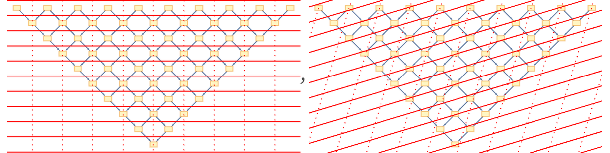
But as a rough idealized picture, we might imagine that we have a causal graph that maintains the same overall structure, but adds some extra connections:

In our actual models, the causal graphs one gets are considerably more complicated. But one can still identify some features from the simple idealization. The basic concept is that energy and momentum add “extra causal connections” that are not “necessary” to define the basic structure of spacetime. In a sense the core thing that defines the structure of spacetime is the way that “elementary light cones” are knitted together.

Consider a causal graph like:

One can think of a set of edges like the ones indicated as in effect “outlining” the causal graph. But then there are other edges that add “extra connections”. The edges that “outline the graph” in effect maximally connect spatially separated regions—or in a sense transmit causal information at a maximum speed. The other edges one can think of as having slower speeds—so they are typically drawn closer to vertical in a rendering like the one above.

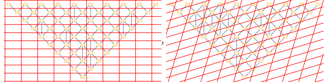
But now let us return to our simple grid idealization of the causal graph—with additional vertical edges added. Now do foliations like the ones we used above to represent inertial frames, parametrized by a velocity ratio β relative to the maximum speed (taken to be 1). Define E(β) to be the density of causal edge crossing of the spacelike hypersurfaces, and p(β) the corresponding quantity for timelike hypersurfaces. Then for speed 1 edges, we have (up to an overall multiplier) (cf. [111][112]):

But in general for edges with speed α we have

which means that for any β

thus showing that our crossing densities transform like energy and momentum for a particle with mass . In other words, we can potentially identify edges that are not maximum speed in the causal graph as corresponding to “matter” with nonzero rest mass. Perhaps not surprisingly, this whole setup is quite analogous to thinking about world lines of massive particles in elementary treatments of relativity.

But in our context, all of this must emerge from underlying features of the evolving hypergraph. Causal connections that transfer information at maximum speed can be thought of as arising from updating events that involve maximally separate nodes, and that are somehow always entraining “fresh” nodes. But causal connections that transfer information more slowly are associated with sequences of updating events that in effect reuse nodes. So in other words, rest mass can be thought of as being associated with local collections of nodes in the hypergraph that allow repeated updating events to occur without the involvement of other nodes.

Given this setup, it is possible to derive other features of energy, momentum and mass by methods similar to those used in typical discussions of relativity. It is first helpful to include units in the quantities we have introduced. If an elementary light cone has timeline extent T then we can consider its spacelike extent to be c T, where c is the speed of light. Within the light cone let us say that there are effectively μ causal edges oriented in the timelike direction. With the inertial frame foliations used above, the contribution of these causal edges to energy and momentum will be (the factor c in the energy case comes from the spacelike extent of the light cone):

But if we define the mass m as and substitute , we get the standard formulas of special relativity [111][112], or to first order

establishing in our model the relation E = m c² between energy and rest mass.

We should note that with our identification for energy and momentum, the conservation of energy becomes essentially the statement that the overall density of events in the causal network does not change as we progress through successive spacelike surfaces. And, as we will discuss later, if in effect the whole hypergraph is in some kind of dynamic equilibrium, then we can reasonably expect that this will be the case. Expansion (or, more specifically, non-uniform expansion) will lead to effective violations of energy conservation, much as it does for an expanding universe in the traditional formalism of general relativity [117][75].

In the previous subsection, we discussed the overall structure of spacetime, and we used the growth rate of the spacetime volume C_t(X) as a way to assess this. But now let us ask about specific values of C_t(X), complete with their “constant” multipliers. We can think of these multipliers as probing the local density of the causal graph. But deviations in this are what we have now identified as being associated with matter.

To compute C_t(X) we ultimately need to be able to precisely count events in the causal graph. If the causal graph is somehow “uniform”, then it cannot contain what can be considered to be “matter”. In the setup we have defined, the presence of matter is effectively associated with “fluxes” of causal edges that reflect the non-uniform “arrangement” of nodes in the causal graph. To represent this, take ρ(X) to be the “local density” of nodes in the causal graph. We can make a series expansion to probe deviations from uniformity in ρ(X). And formally we can write

where the t^μ are timelike vectors used in the definition of C_t and now T_μν is effectively a tensor that represents “fluxes of edges” in the causal graph. But these fluxes are what we have identified as energy and momentum, and when we think about how causal edges traverse spacelike and timelike hypersurfaces, T_μν turns out to correspond exactly to the standard energy-momentum tensor of general relativity.

So now we can combine our formula for the effect of local density with our formula for the effect of curvature from the previous section to get:

But if we apply the same argument as in the previous subsection, then to maintain limiting fixed dimension we get the condition

which has exactly the form of Einstein’s equations in the presence of matter [114][115][75][116].

Just as we interpreted the curvature part of these equations in the previous subsection in terms of the change in area of geodesic bundles, we can interpret the “matter” part in terms of the change of geodesics associated with additional local connections. As an example, consider starting with a 2D hexagonal grid. Now imagine adding edges at each node. Doing this creates additional connections and additional geodesics, eventually producing something like the hyperbolic space examples in 4.2. So what the equation says is that any such effect, which would lead to negative curvature, must be compensated by positive curvature in the “background” spacetime—just as general relativity suggests.