 download pdf
  ARXIV
ARXIV peer review
To continue understanding how our models might relate to quantum mechanics, it is useful to describe a little more of the potential correspondence with standard quantum formalism. We consider—quite directly—each state in the multiway system as some quantum basis state |S>.
An important feature of quantum states is the phenomenon of entanglement—which is effectively a phenomenon of connection or correlation between states. In our setup (as we will see more formally soon), entanglement is basically a reflection of common ancestry of states in the multiway graph. (“Interference” can then be seen as a reflection of merging—and therefore common successors—in the multiway graph.)
Consider the following multiway graph for a string substitution system:
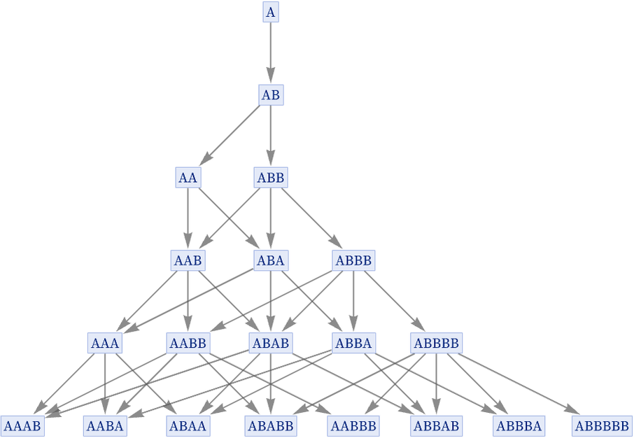
Each pair of states generated by a branching in this graph are considered to be entangled. And when the graph is viewed as defining a rewrite system, these pairs of states can also be said to form a branch pair.
Given a particular foliation of the multiway graph, we can now capture the entanglement of states in each slice of the foliation by forming a branchial graph in which we connect the states in each branch pair. For the string substitution system above, the sequence of branchial graphs is then:
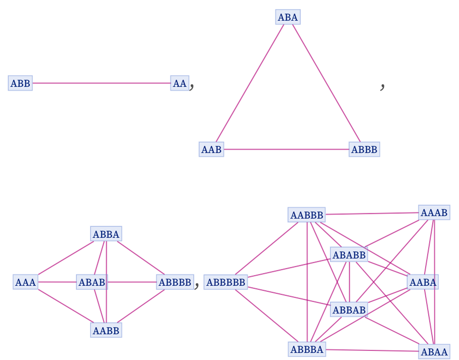
In physical terms, the nodes of the branchial graph are quantum states, and the graph itself forms a kind of map of entanglements between states. In general terms, we expect states that are closer on the branchial graph to be more correlated, and have more entanglement, than ones further away.
As we discussed in 5.17, the geometry of branchial space is not expected to be like the geometry of ordinary space. For example, it will not typically correspond to a finite-dimensional manifold. We can still think of it as a space of some kind that is reached in the limit of a sufficiently large multiway system, with a sufficiently large number of states. And in particular we can imagine—for any given foliation—defining coordinates of some kind on it, that we will denote ![]() . So this means that within a foliation, any state that appears in the multiway system can be assigned a position
. So this means that within a foliation, any state that appears in the multiway system can be assigned a position ![]() in “multiway space”.
in “multiway space”.
In the standard formalism of quantum mechanics, states are thought of as vectors in a Hilbert space, and now these vectors can be made explicit as corresponding to positions in multiway space.
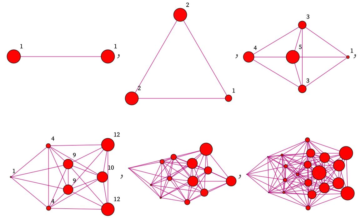
But now there is an additional issue. The multiway system should represent not just all possible states, but also all possible paths leading to states. And this means that we must assign to states a weight that reflects the number of possible paths that can lead to them:

In effect, therefore, each branchlike hypersurface can be thought of as exposing some linear combination of basic states, each one with a certain weight:
Let us say that we want to track what happens to some part of this branchlike hypersurface. Each state undergoes updating events that are represented by edges in the multiway graph. And in general the paths followed in the multiway graph can be thought of as geodesics in multiway space. And to determine what happens to some part of the branchlike hypersurface, we must then follow a bundle of geodesics.
A notable feature of the multiway graph is the presence of branching and merging, and this will cause our bundle of geodesics to diverge and converge. Often in standard quantum formalism we are interested in the projection of one quantum state on another < | >. In our setup, the only truly meaningful computation is of the propagation of a geodesic bundle. But as an approximation to this that should be satisfactory in an appropriate limit, we can use distance between states in multiway space, and computing this in terms of the vectors ![]() the expected Hilbert space norm [122][123] appears:
the expected Hilbert space norm [122][123] appears: ![]() .
.
Time evolution in our system is effectively the propagation of geodesics through the multiway graph. And to work out a transition amplitude <i | S | f> between initial and final states we need to see what happens to a bundle of geodesics that correspond to the initial state as they propagate through the multiway graph. And in particular we want to know the measure (or essentially cross-sectional area) of the geodesic bundle when it intersects the branchlike hypersurface defined by a certain quantum observation frame to detect the final state.
To analyze this, consider a single path in the multiway system, corresponding to a single geodesic. The critical observation is that this path is effectively “turned” in multiway space every time a branching event occurs, essentially just like in the simple example below:
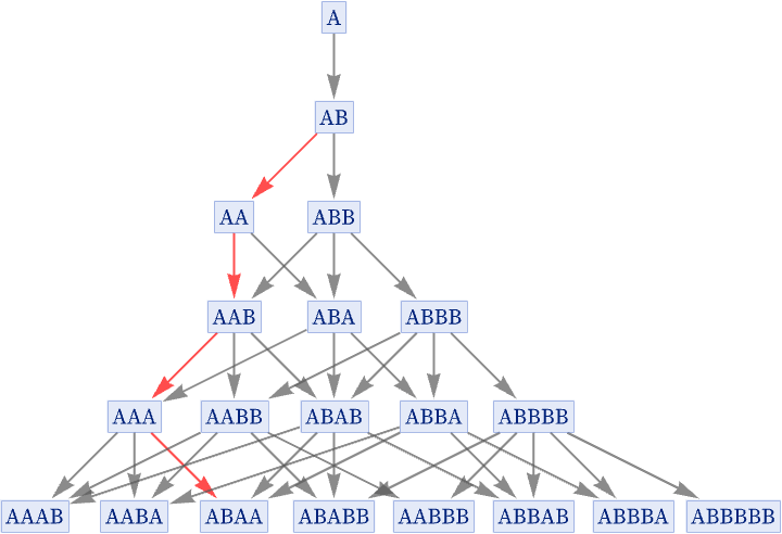
If we think of the turns as being through an angle θ, the way the trajectory projects onto the final branchlike hypersurface can then be represented by ei θ. But to work out the angle θ for a given path, we need to know how much branching there will be in the region of the multiway graph through which it passes.
But now recall that in discussing spacetime we identified the flux of edges through spacelike hypersurfaces in the causal graph as potentially corresponding to energy. The spacetime causal graph, however, is just a projection of the full multiway causal graph, in which branchlike directions have been reduced out. (In a causal invariant system, it does not matter what “direction” this projection is done in; the reduced causal graph is always the same.) But now suppose that in the full multiway causal graph, the flux of edges across spacelike hypersurfaces can still be considered to correspond to energy.
Now note that every node in the multiway causal graph represents some event in the multiway graph. But events are what produce branching—and “turns”—of paths in the multiway graph. So what this suggests is that the amount of turning of a path in the multiway graph should be proportional to energy, multiplied by the number of steps, or effectively the time. In standard quantum formalism, energy is identified with the Hamiltonian H, so what this says is that in our models, we can expect transition amplitudes to have the basic form ei H t—in agreement with the result from quantum mechanics.
To think about this in more detail, we need not just a single energy quantity—corresponding to an overall rate of events—but rather we want a local measure of event rate as a function of location in multiway space. In addition, if we want to compute in a relativistically invariant way, we do not just want the flux of causal edges through spacelike hypersurfaces in some specific foliation. But now we can make a potential identification with standard quantum formalism: we suppose that the Lagrangian density ℒ corresponds to the total flux in all directions (or, in other words, the divergence) of causal edges at each point in multiway space.
But now consider a path in the multiway system going through multiway space. To know how much “turning” to expect in the path, we need in effect to integrate the Lagrangian density along the path (together with the appropriate volume element). And this will give us something of the form ei S, where S is the action. But this is exactly what we see in the standard path integral formulation of quantum mechanics [124].
There are many additional details (see [121]). But the correspondence between our models and the results of standard quantum formalism is notable.
It is worth pointing out that in our models, something like the Lagrangian is ultimately not something that is just inserted from the outside; instead it must emerge from actual rules operating on hypergraphs. In the standard formalism of quantum field theory, the Lagrangian is stated in terms of quantum field operators. And the implication is therefore that the structure of the Lagrangian must somehow emerge as a kind of limit of the underlying discrete system, perhaps a bit like how fluid mechanics can emerge from discrete underlying molecular dynamics (or cellular automata) [110].
One notable feature of standard quantum formalism is the appearance of complex numbers for amplitudes. Here the core concept is the turning of a path in multiway space; the complex numbers arise only as a convenient way to represent the path and understand its projections. But there is an additional way complex numbers can arise. Imagine that we want to put a metric on the full ![]() space of the multiway causal graph. The normal convention for
space of the multiway causal graph. The normal convention for ![]() space is to have real-number coordinates and a norm based on t2 – x2—but an alternative is use i t for time. In extending to
space is to have real-number coordinates and a norm based on t2 – x2—but an alternative is use i t for time. In extending to ![]() space, one might imagine that a natural norm which allows the contributions of t, x and b components to be appropriately distinguished would be t2 – x2 + i b2.
space, one might imagine that a natural norm which allows the contributions of t, x and b components to be appropriately distinguished would be t2 – x2 + i b2.