 download pdf
  ARXIV
ARXIV peer review
Consider the rule:
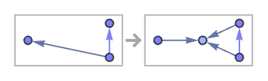
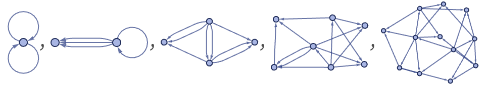
When we discussed this rule previously, we showed the first few steps in its evolution as:
But to understand the updating process in our models in more detail, it is helpful to “look inside” these steps, and see the individual updating events of which they are comprised:
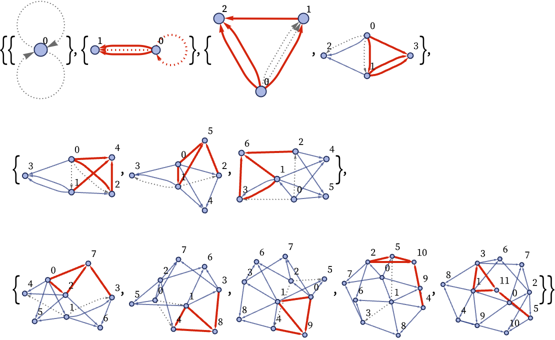
The 22 42 signature of the rule means that in each updating event, two relations are destroyed, and four new ones are created. In the pictures above, new relations from each event are shown in red; the ones that will disappear in the next event are shown dotted. The elements are numbers in the sequence they are created.
There are in general many possible sequences of updating events that are consistent with the rule. But in making the pictures above (and in much of our discussion in previous sections), we have used our “standard updating order”, in which each step in the overall evolution in effect includes as many non-overlapping updates as will “fit”. (In more detail, what is done is that in each overall step, relations are scanned from oldest to newest, in each case using them in an update event so long as this can be done without using any relation that has already been updated in this overall step.)
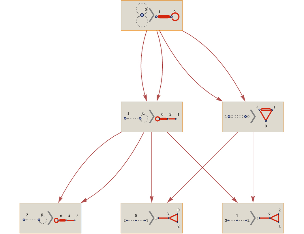
Our models—and the hypergraphs on which they operate—are in many ways more difficult to handle than the string-based systems we discussed in the previous section. But one way in which they are simpler is that they more directly expose causal relationships between events. To see if an event B depends on an event A, all we need do is to see whether elements that were involved in A are also involved in B.
Looking at the sequence of updates above, therefore, we can immediately construct a causal graph:
Another feature of our models is that every element can be thought of as having a unique “lineage”, in that it was created by a particular updating event, which in turn was the result of some other updating event, and so on. When we introduced our models in section 2, we just said that any element created by applying a rule should be new and distinct from all others. If we were implementing the model, this might then make us imagine that the element would have a name based on some global counter, or a UUID.
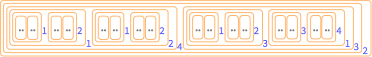
But there is another, more deterministic (as well as more local and distributed) alternative: think of each new element as being a kind of encapsulation of its lineage (analogous to a chain of pointers, or to a hash like in blockchains [84] or Git). In the evolution above, for example, we could describe element 10 by just saying it was created as part of the relation {2,10} from the relations {{2,4},{2,5}} (as the second part of the output of an update that uses them)—but then we could say that these relations were in turn created from earlier relations, and so on recursively, all the way back to the initial state of the system:
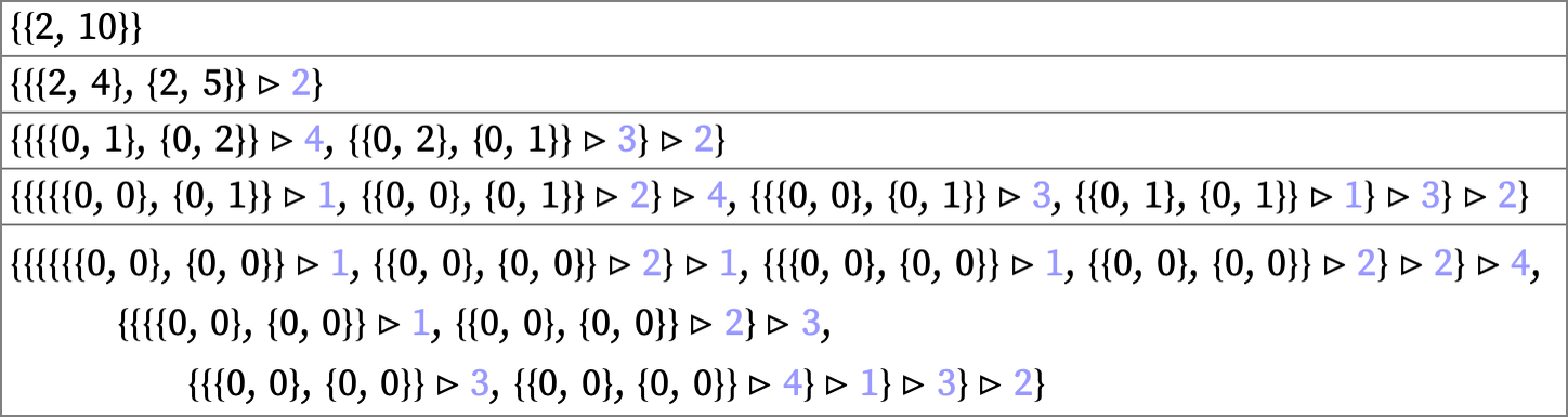
The final expression here can also be written as:
Roughly what this is doing is specifying an element (in this case the one we originally labeled simply as 10) by giving a symbolic representation of the path in the causal graph that led to its creation. And we can then use this to create a unique symbolic name for the element. But while this may be structurally interesting, when it comes to actually using an element as a node in a hypergraph, the name we choose to use for the element is irrelevant; all that matters is what elements are the same, and what are different.