A Class of Models with the Potential to Represent Fundamental Physics
  1. Introduction
  2. Basic Form of Models
  3. Typical Behaviors
  4. Limiting Behavior and Emergent Geometry
  5. The Updating Process for String Substitution Systems
  6. The Updating Process in Our Models
  7. Equivalence and Computation in Our Models
  8. Potential Relation to Physics
  9. Additional Material
  10. References
  11. Index

3.16 The Effect of Initial Conditions

For rules that depend on only a single relation, adding relations to initial conditions always just leads to replication of identical structures, as in these examples for the rule:

{{x, y}} -> {{y, z}, {z, x}}
ResourceFunction["WolframModelPlot"][#, "MaxImageSize" -> 90] & /@ ResourceFunction[ "WolframModel"][{{x, y}} -> {{y, z}, {z, x}}, {{1, 1}}, 5, "StatesList"]

ResourceFunction["WolframModelPlot"][#, "MaxImageSize" -> 180] & /@ ResourceFunction[ "WolframModel"][{{x, y}} -> {{y, z}, {z, x}}, {{1, 1}, {1, 1}}, 5, "StatesList"]

ResourceFunction["WolframModelPlot"][#, "MaxImageSize" -> 100] & /@ ResourceFunction[ "WolframModel"][{{x, y}} -> {{y, z}, {z, x}}, {{1, 1}, {1, 1}, {1, 1}}, 5, "StatesList"]

ResourceFunction["WolframModelPlot"][#, "MaxImageSize" -> 120] & /@ ResourceFunction[ "WolframModel"][{{x, y}} -> {{y, z}, {z, x}}, {{1, 2}, {1, 3}, {1, 5}, {2, 4}, {2, 6}, {3, 4}, {3, 7}, {4, 8}, {5, 6}, {5, 7}, {6, 8}, {7, 8}}, 5, "StatesList"]

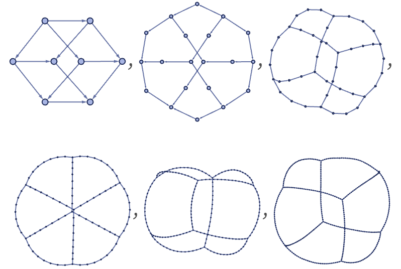
Sometimes, however, the layout of hypergraphs for visualization can make the replication of structures a little less obvious, as in this example for the rule:

{{x, y}} -> {{x, z}, {x, z}, {z, y}}
ResourceFunction["WolframModelPlot"][#, "MaxImageSize" -> 180] & /@ ResourceFunction[ "WolframModel"][{{x, y}} -> {{x, z}, {x, z}, {z, y}}, {{1, 1}}, 5, "StatesList"]

ResourceFunction["WolframModelPlot"][#, "MaxImageSize" -> 180] & /@ ResourceFunction[ "WolframModel"][{{x, y}} -> {{x, z}, {x, z}, {z, y}}, {{1, 1}, {1, 1}}, 5, "StatesList"]

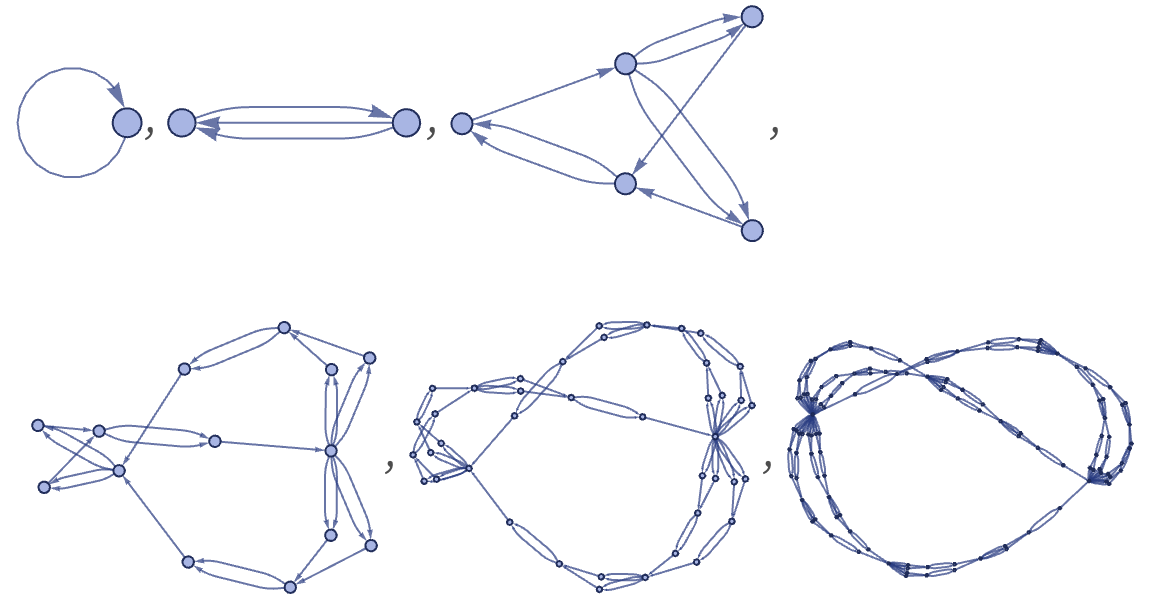
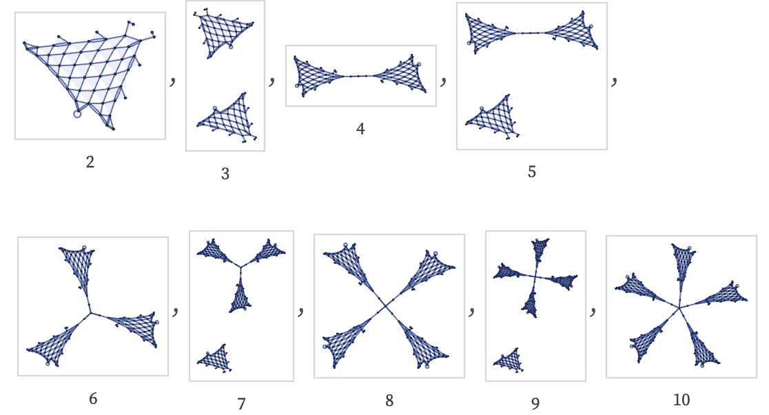
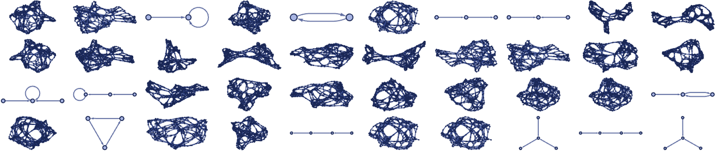
For rules depending on more than one relation, initial conditions can have more important effects. Starting with the rule

{{x, y}, {y, z}} -> {{w, z}, {w, z}, {x, w}, {y, z}}

from all 8 inequivalent 2-relation and all 32 inequivalent 3-relation initial conditions, one sees quite a range of behavior:
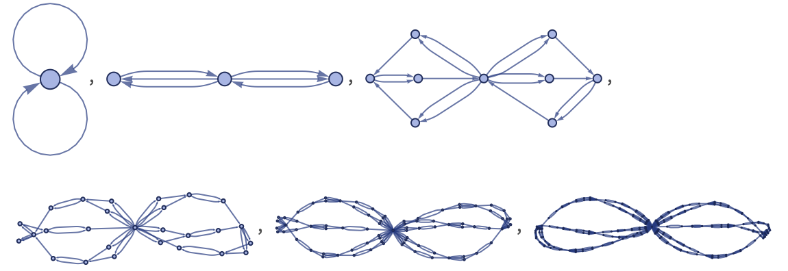
GraphicsGrid[ Partition[ ParallelMap[ ResourceFunction[ "WolframModel"][{{x, y}, {y, z}} -> {{w, z}, {w, z}, {x, w}, {y, z}}, #, 10, "FinalStatePlot"] &, Join[ResourceFunction["EnumerateHypergraphs"][{{2, 2}}], ResourceFunction["EnumerateHypergraphs"][{{3, 2}}]]], 10], ImageSize -> Full]

But in other rulesparticularly many of those such as

{{x, y}, {x, z}} -> {{x, y}, {x, w}, {y, w}, {z, w}}

that yield globular structuresdifferent initial conditions (so long as they lead to growth at all) produce behavior that is different in detail but similar in overall features, a bit like what happens in class 3 cellular automata such as rule 30 [1:p251]):

GraphicsGrid[ Partition[ ParallelMap[ ResourceFunction[ "WolframModel"][{{x, y}, {x, z}} -> {{x, y}, {x, w}, {y, w}, {z, w}}, #, 10, "FinalStatePlot"] &, Join[ResourceFunction["EnumerateHypergraphs"][{{2, 2}}], ResourceFunction["EnumerateHypergraphs"][{{3, 2}}]]], 10], ImageSize -> Full]

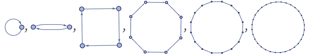
For the evolution of a rule to not just immediately terminate, the left-hand side of the rule must be able to match the initial conditions given (and so must be a sub-hypergraph of the initial conditions). This is guaranteed if the initial conditions are in effect just a copy of the left-hand side. But the most “fertile” initial conditions, with the most possibility for different matches, are always self-loops: in particular, n k-ary self-loops for a rule with signature nk . And in what follows, this is the form of initial conditions that we will most often use.

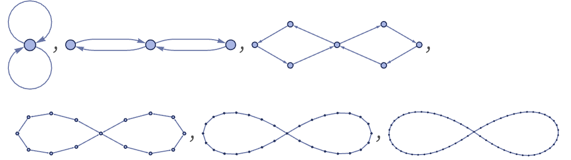
One practical issue with self-loop initial conditions, however, is that they can make it visually more difficult to tell what is going on. Sometimes, for example, initial conditions that lead to slightly less activity, or enforce some particular symmetry, can help. Note, however, that in the evolution of rules that depend on more than one relation, there may be no way to preserve symmetry, at least with any specific updating order (see section 6). Thus, for example, the rule

{{x, y}, {x, z}} -> {{x, y}, {x, w}, {y, w}, {z, w}}

with our standard updating order gives:

gridstart[list_] := Catenate[EdgeList[GridGraph[list]] /. UndirectedEdge[a_, b_] -> {{a, b}, {b, a}}] ResourceFunction[ "WolframModel"][{{x, y}, {x, z}} -> {{x, z}, {x, w}, {y, w}, {z, w}}, gridstart[{4, 4}], 5, "StatesPlotsList"]

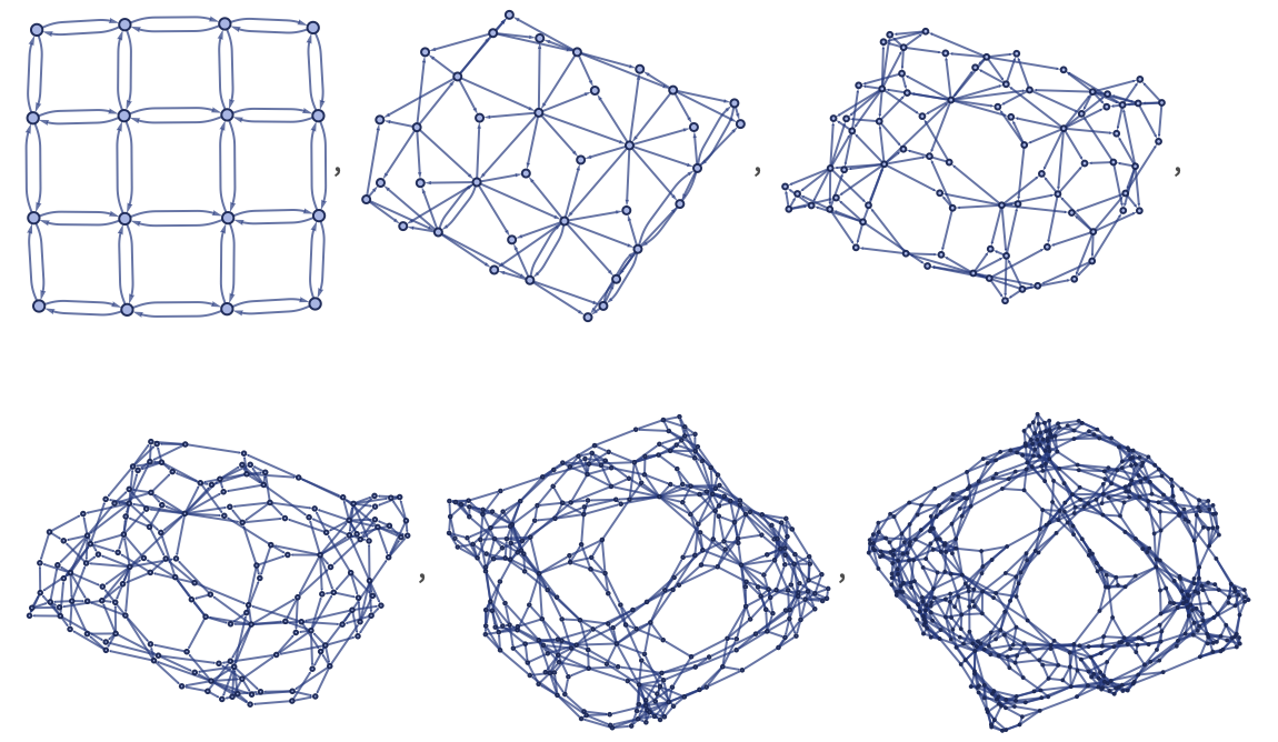
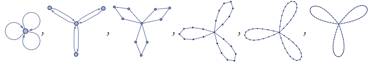
Another feature of initial conditions is that they can affect the connectivity of the results from a rule. Thus, for example, even in the case of the rule above that generates a grid, initial conditions consisting of different numbers of 3-ary self-loops lead to differently connected results:

ParallelTable[ Labeled[Framed[ ResourceFunction["WolframModelPlot"][#, ImageSize -> Tiny], FrameStyle -> LightGray], Text[n, BaseStyle -> {GrayLevel[.25], FontSize -> .85 Inherited, FontFamily -> "Source Serif Pro" }]] &@ ResourceFunction[ "WolframModel"][{{1, 2, 2}, {3, 1, 4}} -> {{2, 5, 2}, {2, 3, 5}, {4, 5, 5}}, Table[{0, 0, 0}, n], 50, "FinalState"], {n, 2, 10}]