A Class of Models with the Potential to Represent Fundamental Physics
  1. Introduction
  2. Basic Form of Models
  3. Typical Behaviors
  4. Limiting Behavior and Emergent Geometry
  5. The Updating Process for String Substitution Systems
  6. The Updating Process in Our Models
  7. Equivalence and Computation in Our Models
  8. Potential Relation to Physics
  9. Additional Material
  10. References
  11. Index

4.9 Adjacency Matrices and Age Distributions

We have made explicit visualizations of the connectivity structures of the graphs (and hypergraphs) generated by our models. But an alternative approach is to look at adjacency matrices (or tensors). In our models, there is a natural way to index the nodes in the graph: the order in which they were created. Here are the adjacency matrices for the first 14 steps in the evolution of the rule {{x,y},{x,z}}{{x,z},{x,w},{y,w},{z,w}} discussed above:

GraphicsGrid[ Partition[ Table[MatrixPlot[ AdjacencyMatrix[ Graph[Rule @@@ ResourceFunction[ "WolframModel"][{{x, y}, {x, z}} -> {{x, z}, {x, w}, {y, w}, {z, w}}, {{1, 2}, {1, 3}}, t, "FinalState"]]], FrameTicks -> None, ImageSize -> Tiny], {t, 0, 14}], 5], ImageSize -> {550, 320}]

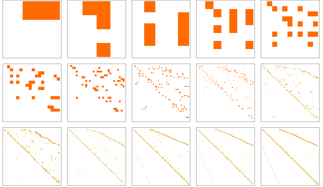
It is notable that even though these adjacency matrices grow by roughly a factor of 1.84 at each step, they maintain many consistent featuresand something similar is seen in many other rules.

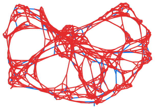
Our models evolve by continually adding new relations, and for example in the rule we are currently considering, there are roughly exponentially more relations at each step. The result, as shown below for step 14, is that at a given step the relations that exist will almost all be from the most recent step (shown in red):

AgeHypergraphPlot[evolutionObject_, gradientList_ : {Red, Blue}, exp_ : .25] := With[{totalGenerationsCount = evolutionObject["TotalGenerationsCount"]}, ResourceFunction["WolframModelPlot"][evolutionObject[-1], EdgeStyle -> Association[ MapThread[#1 -> Directive[Thick, Opacity[.9], Blend[gradientList, 1 - Exp[ exp (#2 - totalGenerationsCount)]]] &, {evolutionObject[ "AllExpressions"], evolutionObject["ExpressionGenerations"]}]], VertexSize -> 0, VertexStyle -> Transparent]]; AgeHypergraphPlot[ ResourceFunction[ "WolframModel"][{{x, y}, {x, z}} -> {{x, z}, {x, w}, {y, w}, {z, w}}, {{1, 2}, {1, 3}}, 12], {Hue[1, 0.81, 0.89], Hue[ 0.5700000000000001, 0.16, 0.86], Hue[0.59, 1, 0.89]}, 5]

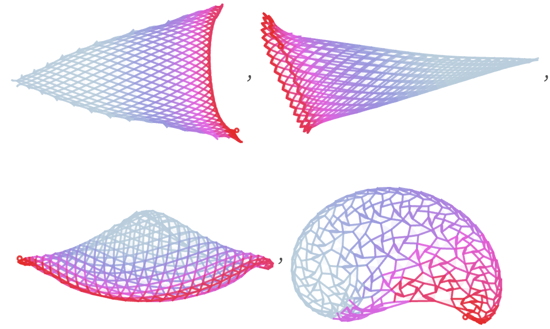
Other rules can show quite different age distributions. Here are age distributions for a few rules that “knit” their structures one relation at a time:

AgeHypergraphPlot[evolutionObject_, gradientList_ : {Red, Blue}, exp_ : .25] := With[{totalGenerationsCount = evolutionObject["TotalGenerationsCount"]}, ResourceFunction["WolframModelPlot"][evolutionObject[-1], EdgeStyle -> Association[ MapThread[#1 -> Directive[Thick, Opacity[.9], Blend[gradientList, 1 - Exp[ exp (#2 - totalGenerationsCount)]]] &, {evolutionObject[ "AllExpressions"], evolutionObject["ExpressionGenerations"]}]], VertexSize -> 0, VertexStyle -> Transparent]]; AgeHypergraphPlot[ ResourceFunction["WolframModel"][#, {{0, 0, 0}, {0, 0, 0}}, 500], {Hue[1, 0.81, 0.89], Hue[0.5700000000000001, 0.16, 0.86], Hue[0.59, 0.15, 0.89]}, .0018] & /@ {{{1, 2, 2}, {3, 1, 4}} -> {{2, 5, 2}, {2, 3, 5}, {4, 5, 5}}, {{1, 1, 2}, {1, 3, 4}} -> {{4, 4, 3}, {2, 5, 3}, {2, 5, 3}}, {{1, 1, 2}, {1, 3, 4}} -> {{4, 4, 5}, {5, 4, 2}, {3, 2, 5}}, {{1, 2, 1}, {1, 3, 4}} -> {{4, 5, 4}, {5, 4, 3}, {1, 2, 5}}}