A Class of Models with the Potential to Represent Fundamental Physics
  1. Introduction
  2. Basic Form of Models
  3. Typical Behaviors
  4. Limiting Behavior and Emergent Geometry
  5. The Updating Process for String Substitution Systems
  6. The Updating Process in Our Models
  7. Equivalence and Computation in Our Models
  8. Potential Relation to Physics
  9. Additional Material
  10. References
  11. Index

4.8 Homogeneity and Local Graph Neighborhoods

In studying Vr we are looking at the total size of the neighborhood up to distance r around a point in a graph. But what about the actual local structure of the neighborhood?

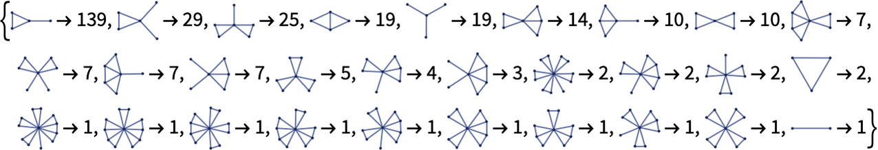
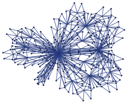
In general, it can be different for every point on the graph. Thus, for example, in

ResourceFunction[ "WolframModel"][{{x, y}, {x, z}} -> {{x, z}, {x, w}, {y, w}, {z, w}}, {{1, 2}, {1, 3}}, 10, "FinalStatePlot"]

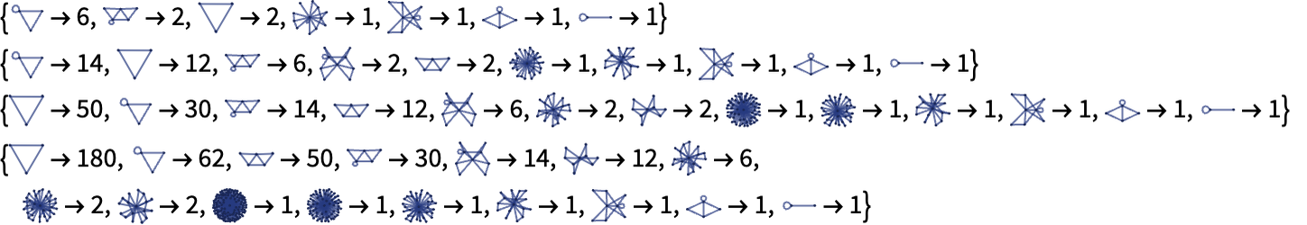
obtained from 10 steps of the rule {{x,y},{x,z}}{{x,z},{x,w},{y,w},{z,w}} the collection of distinct range-1 neighborhoods (with their counts) is:

With[{gr = UndirectedGraph[ Rule @@@ ResourceFunction[ "WolframModel"][{{x, y}, {x, z}} -> {{x, z}, {x, w}, {y, w}, {z, w}}, {{1, 2}, {1, 3}}, 10, "FinalState"]]}, ReverseSortBy[(Graph[CanonicalGraph[First[#]], GraphLayout -> "SpringElectricalEmbedding", VertexCoordinates -> Automatic, ImageSize -> 30, VertexStyle -> ResourceFunction["WolframPhysicsProjectStyleData"][ "SpatialGraph", "VertexStyle"], EdgeStyle -> ResourceFunction["WolframPhysicsProjectStyleData"][ "SpatialGraph", "EdgeLineStyle"]] -> Length[#]) & /@ Gather[NeighborhoodGraph[gr, #, 1] & /@ VertexList[gr], IsomorphicGraphQ], Last]]

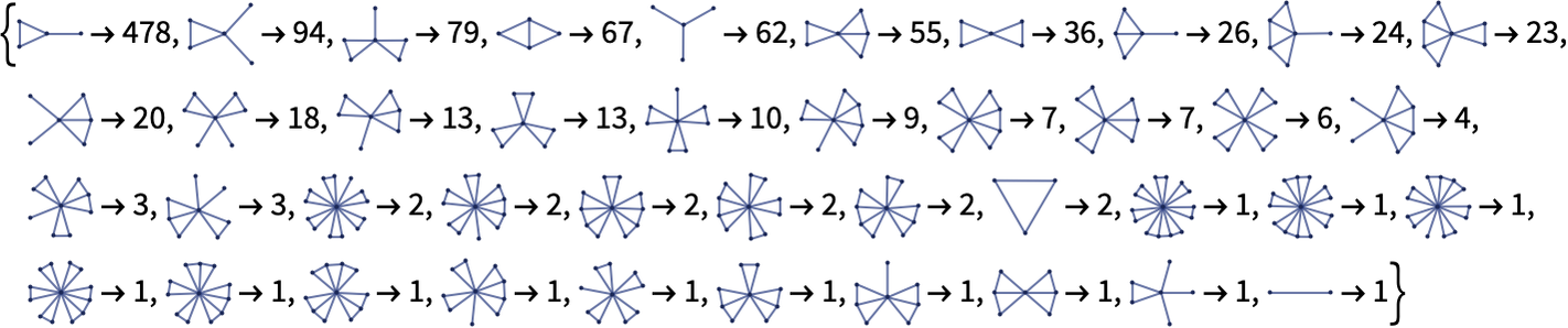
The corresponding result after 12 steps is:

With[{gr = UndirectedGraph[ Rule @@@ ResourceFunction[ "WolframModel"][{{x, y}, {x, z}} -> {{x, z}, {x, w}, {y, w}, {z, w}}, {{1, 2}, {1, 3}}, 12, "FinalState"]]}, ReverseSortBy[(Graph[CanonicalGraph[First[#]], GraphLayout -> "SpringElectricalEmbedding", VertexCoordinates -> Automatic, ImageSize -> 30, VertexStyle -> ResourceFunction["WolframPhysicsProjectStyleData"][ "SpatialGraph", "VertexStyle"], EdgeStyle -> ResourceFunction["WolframPhysicsProjectStyleData"][ "SpatialGraph", "EdgeLineStyle"]] -> Length[#]) & /@ Gather[NeighborhoodGraph[gr, #, 1] & /@ VertexList[gr], IsomorphicGraphQ], Last]]

And it seems that for this rule the distribution of different forms for a given range of neighborhood generally stabilizes as the number of steps increases. (It may be possible to characterize it as limiting to an invariant measure in the space of possible hypergraphs, perhaps with some related entropy (cf. [1:p958][31]).)

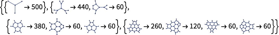
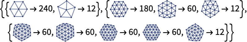
One sees the same kind of stabilization for most rules, though, for example, in a case like

ResourceFunction[ "WolframModel"][{{x, y}} -> {{x, y}, {y, z}, {z, x}}, {{1, 1}}, 6, "FinalStatePlot"]

from the rule {{x,y}}{{x,y},{y,z},{z,x}} one always gets some neighborhoods with new forms at each step:

Column[Table[ With[{gr = UndirectedGraph[ Rule @@@ ResourceFunction[ "WolframModel"][{{x, y}} -> {{x, y}, {y, z}, {z, x}}, {{1, 1}}, t, "FinalState"]]}, ReverseSortBy[(Graph[CanonicalGraph[First[#]], GraphLayout -> "SpringElectricalEmbedding", VertexCoordinates -> Automatic, ImageSize -> 20, VertexStyle -> ResourceFunction["WolframPhysicsProjectStyleData"][ "SpatialGraph", "VertexStyle"], EdgeStyle -> ResourceFunction["WolframPhysicsProjectStyleData"][ "SpatialGraph", "EdgeLineStyle"]] -> Length[#]) & /@ Gather[NeighborhoodGraph[gr, #, 1] & /@ VertexList[gr], IsomorphicGraphQ], Last]], {t, 3, 6}]]

In general, the presence of many identical neighborhoods reflects a certain kind of approximate symmetry or isometry of the emergent geometry of the system.

In a torus graph, for example, the symmetry is exact, and all local neighborhoods of a given range are the same:

Table[With[{gr = ResourceFunction["TorusGraph"][{5, 5}]}, (Graph[ CanonicalGraph[First[#]], GraphLayout -> "SpringElectricalEmbedding", VertexCoordinates -> Automatic, ImageSize -> 40, VertexStyle -> ResourceFunction["WolframPhysicsProjectStyleData"][ "SpatialGraph", "VertexStyle"], EdgeStyle -> ResourceFunction["WolframPhysicsProjectStyleData"][ "SpatialGraph", "EdgeLineStyle"]]) & /@ Gather[NeighborhoodGraph[gr, #, r] & /@ VertexList[gr], IsomorphicGraphQ]], {r, 5}]

The same is true for a 3D torus graph:

Table[With[{gr = ResourceFunction["TorusGraph"][{5, 5, 5}]}, (Graph[ CanonicalGraph[First[#]], GraphLayout -> "SpringElectricalEmbedding", VertexCoordinates -> Automatic, ImageSize -> 40, VertexStyle -> ResourceFunction["WolframPhysicsProjectStyleData"][ "SpatialGraph", "VertexStyle"], EdgeStyle -> ResourceFunction["WolframPhysicsProjectStyleData"][ "SpatialGraph", "EdgeLineStyle"]]) & /@ Gather[NeighborhoodGraph[gr, #, r] & /@ VertexList[gr], IsomorphicGraphQ]], {r, 5}]

For a sphere graph not every point has the exact same local neighborhood, but there are a limited number of neighborhoods of a given range:

Table[With[{gr = ResourceFunction["BuckyballGraph"][4]}, ReverseSortBy[(Graph[CanonicalGraph[First[#]], GraphLayout -> "SpringElectricalEmbedding", VertexCoordinates -> Automatic, ImageSize -> 30, VertexStyle -> ResourceFunction["WolframPhysicsProjectStyleData"][ "SpatialGraph", "VertexStyle"], EdgeStyle -> ResourceFunction["WolframPhysicsProjectStyleData"][ "SpatialGraph", "EdgeLineStyle"]] -> Length[#]) & /@ Gather[NeighborhoodGraph[gr, #, r] & /@ VertexList[gr], IsomorphicGraphQ], Last]], {r, 4}]

And from the dual graph it becomes clear that these are associated with hexagonal and pentagonal “faces”:

Table[With[{ms = Graph[{1, 2, 3, 4, 5, 6, 7, 8, 9, 10, 11, 12, 13, 14, 15, 16, 17, 18, 19, 20, 21, 22, 23, 24, 25, 26, 27, 28, 29, 30, 31, 32, 33, 34, 35, 36, 37, 38, 39, 40, 41, 42, 43, 44, 45, 46, 47, 48, 49, 50, 51, 52, 53, 54, 55, 56, 57, 58, 59, 60, 61, 62, 63, 64, 65, 66, 67, 68, 69, 70, 71, 72, 73, 74, 75, 76, 77, 78, 79, 80, 81, 82, 83, 84, 85, 86, 87, 88, 89, 90, 91, 92, 93, 94, 95, 96, 97, 98, 99, 100, 101, 102, 103, 104, 105, 106, 107, 108, 109, 110, 111, 112, 113, 114, 115, 116, 117, 118, 119, 120, 121, 122, 123, 124, 125, 126, 127, 128, 129, 130, 131, 132, 133, 134, 135, 136, 137, 138, 139, 140, 141, 142, 143, 144, 145, 146, 147, 148, 149, 150, 151, 152, 153, 154, 155, 156, 157, 158, 159, 160, 161, 162, 163, 164, 165, 166, 167, 168, 169, 170, 171, 172, 173, 174, 175, 176, 177, 178, 179, 180, 181, 182, 183, 184, 185, 186, 187, 188, 189, 190, 191, 192, 193, 194, 195, 196, 197, 198, 199, 200, 201, 202, 203, 204, 205, 206, 207, 208, 209, 210, 211, 212, 213, 214, 215, 216, 217, 218, 219, 220, 221, 222, 223, 224, 225, 226, 227, 228, 229, 230, 231, 232, 233, 234, 235, 236, 237, 238, 239, 240, 241, 242, 243, 244, 245, 246, 247, 248, 249, 250, 251, 252}, { Null, CompressedData[" 1:eJwB7QUS+iFib1JiAgAAAO4CAAACAAAAAQMDAgIBBAMBBAMFBQIGAQIGBwME BwEICAQDCQkFCgIFCgsBBgsCDAwGBwkEDQ0HDgUJDgcPDwkLCBAECBAKDAUR EQoGEhILEwYMExQICxQKFRUMEA0WBw0WDhEJFxcOFg8PFwgYGBAZChEZGg0Q Gg4bGxETEhwLEhwMHR0THg8WHh4XDR8fFiAOFyAUGBwUGRUVHSESEyEiEBgi ESMjGRQkJBglFRklEiYmHCcTHScoFBwoFSkpHRYqKh4rFx4rGh8iGiAbGyMf KisgISYnIRosLB8tGyAtGC4uIi8ZIy8wGiIwGzExIzIeKjIyKygkHDMzKCUp NB0pNCYzNCckLi8lHzU1KjYgKzYhNzcmOCEnOCg5OSQ6KSU6OyIuOyM8PC8z OTo0JD09Lj4lLz4mPz8zQCc0QCpBQTJCKzJCMCwsNS0xNi07MDE8NUFCNjk9 Pjo4Nzc/QDhDLDBDLUREMSxFRTVGLTZGM0dHOUg0OkguSUk7Si88Sj1JSj5L MkFLS0I/R0hATDA7TDFNTTw1Tk5BTzZCT1A3OFA5UVE9Ujo+UjdTUz9UOEBU R1FSSENFTENGRERNRU5PRj9VVUdWQEhWVztJVzxYWEo9WVlJWj5KWkFbW0tc QktcV0xNWFFZWlJDXV1FXkRGXk5bXE9QU1RQX0NMX0RgYE1HYWFRYkhSYlNV VlRFY2NOZEZPZEllZVdmSlhmVWFiVlllZlpnTFdnTWhoWFBpaVNqUFRqa0tb a2tcUWxsWW1SWm1Obm5bb09cb1NwcFVxVFZxX11nX15gYGhdY2ReYWxtYlVy cmFzVmJzY25vZF90dF11YF51dldldlh3d2ZZeHhleVpmeXZnaHdbenpre1xr e2d0dWhdfHxjfV5kfWppaXBxamx4eW1uentvYX5+bH9ibX9wcnNxY4CAboFk b4GCaWqCdHx9dWmDg3CEanGEcn5/c2eFhXSGaHWGdoWGd2WHh3aIZneIiWt6 iYl7eIeIeWyKiniLbXmLfICBfW6MjHqNb3uNcI6Oco9xc490kJB8kXV9kX6K i3+Cg4SCgIyNgXqSkomTe4mTcpSUfpVzf5WFkJGGdpaWhZd3hpeDjo+EfJiY gJl9gZmHlpeIeJqah5t5iJuCnJyDhJyKmpuLjJKTjX6dnYqef4uejpSVj4Cf n4yggY2gkJiZkYOhoY6ihI+ihaOjkKSGkaSSk5ajpJeHpaWWpoiXppSdnpWM p6eSqI2TqJqlppuKqamaqoubqpifoJmcoaKcjqurlKyPlaySra2TkK6umK+R ma+dqaqen6eooKGrrKKUsLCdsZWesaOur6SWsrKjs5eks5y0tKGitKWys6aa tbWltpumtqm1tqqYt7efuJmguKetraidubmpup6ququwsayfu7unvKCovK63 uK+hvb2rvqKsvqO/v67ApK/Ap8HBrcKorcKwubqxubW2urS9vrTDpbXDpsTE trK/wLPDsrPEq8XFsMassca3u7y4rsfHt8ivuMiwycm5yrG6ysu1ucu2zMy6 u8HCvL3Fxr6/x8jAtM3Nvb7NwcLLw8TMss7Ov8+zwM+30NC70bi80cPOz8TF ycrGu9LSwdO8wtPH0NHIycvMysHU1MK91dXF1r7G1r/X18fYwMjY2cPL2cTa 2szN1dbNztfYz9nOz9rQ0tPRxdvbydzGytzdy8ndzN7eysff39DgyNHg0tTU 09ff4NjV29zW3dna3tDh4dLi0dPizePj1dbjzuTk1+XP2OXZ5OXa3+Hi4Nvd 3tzS5ubU59PU59fo6N/p2ODp1erq2+vW3Ovs2d3s2u3t3tvu7t3v3N7v4+rr 4+Hm5+Lk6Onl6OHi6ezk5e3m5+ru7+vk8PDo8eXp8eHy8ubz4ufz6PLz6eP0 9Orr9O7s7e/s8PHt5vX15+r29u736+/3+Ozu+O35+e/09vf08PLz8fL19fP4 8PH5+vLw+vP7+/H2+Pn39/b69fX7+Pr7+fz29/z8+Pn8+vv8+vv8xx3nrQ== "]}, {FormatType -> TraditionalForm}]}, Normal[KeyMap[ Graph[#, ImageSize -> 30, VertexStyle -> ResourceFunction["WolframPhysicsProjectStyleData"][ "SpatialGraph", "VertexStyle"], EdgeStyle -> ResourceFunction["WolframPhysicsProjectStyleData"][ "SpatialGraph", "EdgeLineStyle"]] &, ReverseSort@ Counts[ParallelMap[CanonicalGraph, ParallelMap[NeighborhoodGraph[ms, #, r] &, VertexList[ms]]]]]]], {r, 1, 3}]

For a (spherical) Sierpiński graph, there are also a limited number of neighborhoods of a given range:

Table[With[{gr = \!\(\* GraphicsBox[ NamespaceBox["NetworkGraphics", DynamicModuleBox[{Typeset`graph = HoldComplete[ Graph[CompressedData[" 1:eJwt0NFGgwEAgNG/JEmSSZJJJZNMkiQz6Rl6hC6TlSSTJEmSJEmSJEmSJEmS JJkkSTJJkiRJkiRJks5FF8d3/5W3drQkMoIgaKftvwk66aKbHpL00kc/Awwy xDAjjDLGOBNMMsU0M8wyxzwLLLLEMiusssY6G2yyxTY77LLHPgcckuKIY044 5YxzLkhzyRXX3HDLHfc88MgTz7zwyhvvfPDJF9/88EtgWiZZZJNDLnnkU0CI QooopoQwpZRRQSURqqgmSg211FFPA43EiNNEM3+nCjsd "], { Null, CompressedData[" 1:eJwVxVWSggAAAFAFO0BsMVEs7E4sUOzAbsVGZ7zTnnR3P948jPuyHCAQCH7+ /C8EhCAAisQiiVgiFEllUrlMDkjFMoVSoVKqQJUaUsMQrFBrEI0W0So1EKLT 6wx6g8RgNBnNJrPOCJstqMWKWvUWE2qz2xx2h9PlxFyYzen2uHEPbne7PHLc 6/P6fX6HPxAMEEHCGwiFQ5FwxBcKhqOxaDwWx+KJZCKVTEUTRCqdSWcz2Vg6 mcnlc4V8oVgqlkvlXJGskNVKNU+WKtpqrV5r1BuFBkVTTbpZo1pMq8206y2a ibQ73U6v2yv3+oP+cDDs9JvD0Xg0GU+6o8GYnbKz6Wy+mC8XS3a+Wq826810 tVhbN9vddr/bz/aH4+F0PG0PZ+584S6785HLXq636/12X94fz8fr+bo+Ti/+ zX/enxv/fE8+v6+5R0c= "]}, { GraphLayout -> "TutteEmbedding", ImageSize -> Tiny, VertexSize -> {Tiny}}]]}, TagBox[GraphicsGroupBox[GraphicsComplexBox[CompressedData[" 1:eJxVU3s01HkU98jIqpCoyInGs0gPkjyuooeTlJQebISxlVAeRS1CHiGEkBBK hfImLF2UvF/DJCYZMx4TRtmabEp2N7/Zc/ae8z33n+/n3M+9n89Hwd7tMEWA j4/v/D/v3+6golbb5FUGWdf0PPfLTcEv4Wlmuj45VXw/6yPEkOJqfWM6QQr3 7R1gT8FK4Ru9579cBG2DuehFbhPA4paSr0WX4fBQJdlQdAI4U6tV7DECDGjL KgMV30PqAh4lCbxtAC3JU4KK2gebZLdETcKin3MY+NjsOPtK2QSgTNsDkYMs uJBdVx6ydwza9Pyd0tJH/+vzP2sQnhD/xa2pd/zMWBBWR7O64s8Cu3UsS5rc CAjyixiJKAyBX1exYKr3EISuG88fkGJCDoETXJgLdmLqAY7x48AQ0HEOvkuH FQTP28TeM0ymOf1xI/gLHJ8CMguGkm6t/3GqHl6zdx0ViWUCXcKkerAXIfT2 9nnjT8Ngm5dn3n2MCgNSiRSX4SGgWUWGk0qosNTVdfwjmwHi27elk+Z7oTNy dl4yYwjiGFlOm8MaYE5O21EVBmF+kuPuFd4C9+VfzyWfewdBpqTT5Px6SDpW u7x2Yz8MmohwEjo5mBS2crHLkZcgvcAXQwm+hG4obLNiq/LDwirHs2vcxsLG 8Sg71d/0bQtMO5Xon3Z8j+XFjydj3bth67msmWoKG4Pf5SqbWDdC3sJ98BNx Z5/ZoI1+hu9RO3TP5xk5BrQv6IAthB7+ueTiV1cn8OrBGYt9Rn2YTeB5uhK6 Yxrhgw8H1Pq+dY+hlIGTgc0mOuo5X1ybJTCKlhbcc4acQaTpad4MnRvBBzY7 i2Ic3mATMa+H6E90DvU6bxvGCoqsOnv1KH5f4Ik83oVnuq+6rBjGsE/vf7UX SMdgTeO8RxYs1HELptsmh6B3rqHotPEITpR/qbXZmQ1jAhLS+Y9YGP3bdq1o dg0GT1f2Z9cwUU+Zlc5Jq8OaSkt/rsIwCrsMVmvJtKKldZVQUgoDxc60kfm2 5uBj97O+x70Z+LtKzH3VklJcdUnRK2rlW0wkBbicC3+Kwews5uKnbBDtFfZc 5DuEuYT/eLx5vm4l9vOgLXfmLxiDt/FK3HdP6Gh5vSs1tIcNd0IkGy+ovsaj 1q0fPKJGQNXVla003Ie8XN4g7tvmXJyhAByoWexGutfZhLwcL/ghQ1/q8g6K hCANKo7ob/O3mcT4/+cbebkg8oii43fJLtOt4MnSmlG6NI7khI6cr6trwUhm jcNk3zgmBl8o2FDSAmJ/pjwUVmcTvrulz/MhmHrIPz2VhY2pClFJExwMJ3jy fOuzKtY8cbYfLKUHaXEdA+hodCnbvasfpiMOLy3tomNi4O6vVGUGKBaETyn2 0nHkeX5OXicN6PVPW7lMBnp5z4qNTXUDO6G+esVNBi7x2x8SFUaF6ZcnxUla LBxoLHghq04DdoSPtGt7H8rFdQv5eHRDXECGXaQ8Hc2shH6cgS5oWGK8SdLn NeaqpnHXpdwBqbV1GnsyKuDQ/NJK1TX34BuFOmqlVgPOXhWB1CUB+KE9Vj5z tBRMC5NtL67NBcUTtkrSOWVwQjbfPe1wIQRdEDX3OlUFmvuZJyO5BRC0rKLD 73su3Oho2FshVgxcK9UxzrNG4AiouN1zLwUNbe3n9rqN0KOQ7RvO/QO22ypd 9mZ2wlxtvp2lfSU6XG80r9c8BSIWYW+OJNdg+qfUBB3+8wAhRfIDsSXou+GE se58Gqxdz9pMsa1ArQJJfZk3KViOpNUudMTFe1wgsSoTHdOFmimMQrQLtPBL 8clGi2B2w+kjzThsaa3RY5+AH5VGnuiqNaPByx0SWYfSMc51I6VpDRU5yuRQ 1UX38cCz3visz0VwNW65gdTBIiSzOmReiZdD14v7Z+felKH2jEbe4R/FUBg+ qsaUzcRvg04mranZUOux0qSK9Az5kveJDlXlg0eEGv96cjXuNts0q94WCQpG ZHX9zFLcTO2ILrxXAzfraetlE1+ioKZyW/sWhDnDXc2OdvW4akvHIXODV1Bc otUQ+Vcr/g1cwYVH "], { {Hue[0.6, 0.7, 0.5], Opacity[0.7], LineBox[CompressedData[" 1:eJwVxVWSggAAAFAFO0BsMVEs7E4sUOzAbsVGZ7zTnnR3P948jPuyHCAQCH7+ /C8EhKBQBICAFFSJxCKJWCKWSQxSmVQuk8txhVKhUqiVKqVGDalhCIYQ2KxB NFpEq63q9DqDzqg36C1Gk9FsMptQC2qxolbrxma3OWxOu8PudvidLifmwlwe LO72uHEP7vV5/d6Az+8LBYIBIkgEw0QqFA5FwpFIOxqLxqOJWDyWTiQTqWQq mUln0tlMNnvJ5XOFXDFfyJOFRrFULJfKpUq5R1bIaqVaq9caNareqLcommrS TZppDltMq820O91Or9Pv9rqj/qA/HAwH49F4NBlPJh92ys7Y+XQ2Xc3288V8 uVgu1sv7ar3arDfb3Xa/Pez2u/PheDgdT0fu9Dpz5wt3ud6u9+vjdr/xj+fj 9Xw93/yb/7w/v6kFR0c= "]]}, {Hue[0.6, 0.2, 0.8], EdgeForm[{GrayLevel[0], Opacity[0.7]}], DiskBox[1, 0.0002522464934702044], DiskBox[2, 0.0002522464934702044], DiskBox[3, 0.0002522464934702044], DiskBox[4, 0.0002522464934702044], DiskBox[5, 0.0002522464934702044], DiskBox[6, 0.0002522464934702044], DiskBox[7, 0.0002522464934702044], DiskBox[8, 0.0002522464934702044], DiskBox[9, 0.0002522464934702044], DiskBox[10, 0.0002522464934702044], DiskBox[11, 0.0002522464934702044], DiskBox[12, 0.0002522464934702044], DiskBox[13, 0.0002522464934702044], DiskBox[14, 0.0002522464934702044], DiskBox[15, 0.0002522464934702044], DiskBox[16, 0.0002522464934702044], DiskBox[17, 0.0002522464934702044], DiskBox[18, 0.0002522464934702044], DiskBox[19, 0.0002522464934702044], DiskBox[20, 0.0002522464934702044], DiskBox[21, 0.0002522464934702044], DiskBox[22, 0.0002522464934702044], DiskBox[23, 0.0002522464934702044], DiskBox[24, 0.0002522464934702044], DiskBox[25, 0.0002522464934702044], DiskBox[26, 0.0002522464934702044], DiskBox[27, 0.0002522464934702044], DiskBox[28, 0.0002522464934702044], DiskBox[29, 0.0002522464934702044], DiskBox[30, 0.0002522464934702044], DiskBox[31, 0.0002522464934702044], DiskBox[32, 0.0002522464934702044], DiskBox[33, 0.0002522464934702044], DiskBox[34, 0.0002522464934702044], DiskBox[35, 0.0002522464934702044], DiskBox[36, 0.0002522464934702044], DiskBox[37, 0.0002522464934702044], DiskBox[38, 0.0002522464934702044], DiskBox[39, 0.0002522464934702044], DiskBox[40, 0.0002522464934702044], DiskBox[41, 0.0002522464934702044], DiskBox[42, 0.0002522464934702044], DiskBox[43, 0.0002522464934702044], DiskBox[44, 0.0002522464934702044], DiskBox[45, 0.0002522464934702044], DiskBox[46, 0.0002522464934702044], DiskBox[47, 0.0002522464934702044], DiskBox[48, 0.0002522464934702044], DiskBox[49, 0.0002522464934702044], DiskBox[50, 0.0002522464934702044], DiskBox[51, 0.0002522464934702044], DiskBox[52, 0.0002522464934702044], DiskBox[53, 0.0002522464934702044], DiskBox[54, 0.0002522464934702044], DiskBox[55, 0.0002522464934702044], DiskBox[56, 0.0002522464934702044], DiskBox[57, 0.0002522464934702044], DiskBox[58, 0.0002522464934702044], DiskBox[59, 0.0002522464934702044], DiskBox[60, 0.0002522464934702044], DiskBox[61, 0.0002522464934702044], DiskBox[62, 0.0002522464934702044], DiskBox[63, 0.0002522464934702044], DiskBox[64, 0.0002522464934702044], DiskBox[65, 0.0002522464934702044], DiskBox[66, 0.0002522464934702044], DiskBox[67, 0.0002522464934702044], DiskBox[68, 0.0002522464934702044], DiskBox[69, 0.0002522464934702044], DiskBox[70, 0.0002522464934702044], DiskBox[71, 0.0002522464934702044], DiskBox[72, 0.0002522464934702044], DiskBox[73, 0.0002522464934702044], DiskBox[74, 0.0002522464934702044], DiskBox[75, 0.0002522464934702044], DiskBox[76, 0.0002522464934702044], DiskBox[77, 0.0002522464934702044], DiskBox[78, 0.0002522464934702044], DiskBox[79, 0.0002522464934702044], DiskBox[80, 0.0002522464934702044], DiskBox[81, 0.0002522464934702044], DiskBox[82, 0.0002522464934702044], DiskBox[83, 0.0002522464934702044], DiskBox[84, 0.0002522464934702044], DiskBox[85, 0.0002522464934702044], DiskBox[86, 0.0002522464934702044], DiskBox[87, 0.0002522464934702044], DiskBox[88, 0.0002522464934702044], DiskBox[89, 0.0002522464934702044], DiskBox[90, 0.0002522464934702044], DiskBox[91, 0.0002522464934702044], DiskBox[92, 0.0002522464934702044], DiskBox[93, 0.0002522464934702044], DiskBox[94, 0.0002522464934702044], DiskBox[95, 0.0002522464934702044], DiskBox[96, 0.0002522464934702044], DiskBox[97, 0.0002522464934702044], DiskBox[98, 0.0002522464934702044], DiskBox[99, 0.0002522464934702044], DiskBox[100, 0.0002522464934702044], DiskBox[101, 0.0002522464934702044], DiskBox[102, 0.0002522464934702044], DiskBox[103, 0.0002522464934702044], DiskBox[104, 0.0002522464934702044], DiskBox[105, 0.0002522464934702044], DiskBox[106, 0.0002522464934702044], DiskBox[107, 0.0002522464934702044], DiskBox[108, 0.0002522464934702044]}}]], MouseAppearanceTag["NetworkGraphics"]], AllowKernelInitialization->False]], DefaultBaseStyle->{ "NetworkGraphics", FrontEnd`GraphicsHighlightColor -> Hue[0.8, 1., 0.6]}, FormatType->TraditionalForm, FrameTicks->None, ImageSize->Tiny]\)}, ReverseSortBy[(Graph[CanonicalGraph[First[#]], GraphLayout -> "SpringElectricalEmbedding", VertexCoordinates -> Automatic, ImageSize -> 40] -> Length[#]) & /@ Gather[NeighborhoodGraph[gr, #, r] & /@ VertexList[gr], IsomorphicGraphQ], Last]], {r, 4}]

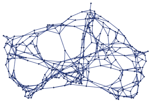
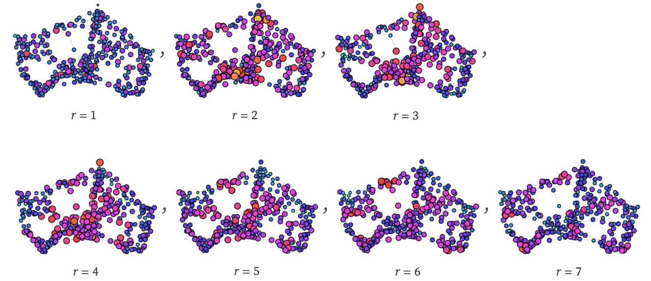
Whenever every local neighborhood is essentially identical, Vr(X) will have the same form for every point X in a graph or hypergraph. But in general Vr(X) (and the log differences Δr(X)) will depend on X. The picture below shows the relative values of Δr(X) at each point in the structure we showed above:

LDLocalGraph[g_, r_, opts___] := With[{ld = N[ResourceFunction["LogDifferences"] /@ ResourceFunction["GraphNeighborhoodVolumes"][UndirectedGraph[g], All, Automatic]]}, Graph[g, VertexStyle -> (# -> Hue[.24 (ld[#][[r]]) + .12, .7, .9] & /@ VertexList[g]), EdgeStyle -> LightGray, opts, VertexSize -> ((# -> 2 ld[#][[r]]) & /@ VertexList[g]), PlotTheme -> "Default"]] With[{gg = Graph[Rule @@@ ResourceFunction[ "WolframModel"][{{x, y}, {x, z}} -> {{x, z}, {x, w}, {y, w}, {z, w}}, {{1, 2}, {1, 3}}, 10, "FinalState"]]}, Table[Labeled[LDLocalGraph[gg, r, ImageSize -> 150], Text[Style[Row[{Style["r", Italic], StringTemplate[" = ``"][r]}], Directive[GrayLevel[.25], FontSize -> .85 Inherited, FontFamily -> "Source Serif Pro"]]]], {r, 7}]]

We can also compute the distribution of values for Δr(X) across the structure, as a function of r:

FullLDList[g_] := N[ResourceFunction["LogDifferences"] /@ ResourceFunction["HypergraphNeighborhoodVolumes"][g, All, Automatic]]; Module[{r = 1}, Histogram[#, PlotRange -> {{0, 4.5}, Automatic}, Frame -> True, FrameTicks -> {Automatic, None}, ImageSize -> Tiny, Epilog -> Text[Style[ Row[{Style["r", Italic], StringTemplate[" = ``"][r++]}], Directive[FontSize -> 12, GrayLevel[0.2], FontFamily -> "Source Serif Pro"]], Scaled[{0, 1}], {-1.3, 1.1}]] & /@ Transpose[ Values[FullLDList[ ResourceFunction[ "WolframModel"][{{x, y}, {x, z}} -> {{x, z}, {x, w}, {y, w}, {z, w}}, {{1, 2}, {1, 3}}, 10, "FinalState"]]]]]

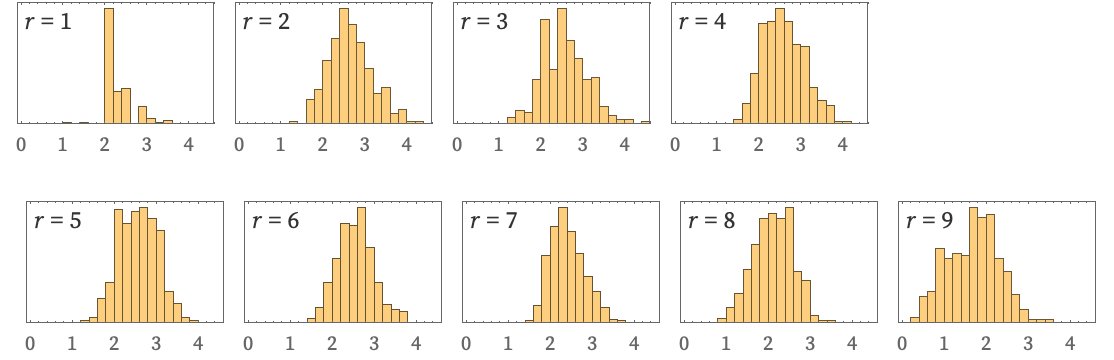
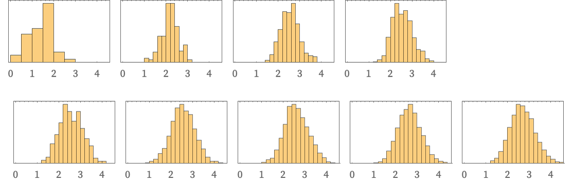
Both these pictures indicate a certain statistical uniformity in Vr(X). This is also seen if we look at the evolution of the distribution of Δr(X), here shown for the specific value r = 6, for steps 8 through 16:

FullLDList[g_] := N[ResourceFunction["LogDifferences"] /@ ResourceFunction["HypergraphNeighborhoodVolumes"][g, All, Automatic]]; Table[Histogram[#, PlotRange -> {{0, 4.5}, Automatic}, Frame -> True, FrameTicks -> {Automatic, None}, ImageSize -> Tiny] &@ Transpose[ Values[FullLDList[ ResourceFunction[ "WolframModel"][{{x, y}, {x, z}} -> {{x, z}, {x, w}, {y, w}, {z, w}}, {{1, 2}, {1, 3}}, t, "FinalState"]]]][[6]], {t, 8, 16}]