4.7 Curvature

In ordinary plane geometry, the area of a circle is πr². But if the circle is drawn on the surface of a sphere of radius a, the area of the spherical region enclosed by the circle is instead:

In other words, curvature in the underlying space introduces a correction to the growth rate for the area of the circle as a function of radius. And in general there is a similar correction for the volume of a d-dimensional ball in a curved space (e.g. [24][1:p1050])

where here R is the Ricci scalar curvature of the space [25][26][27]. (For example, for the d-dimensional surface of a (d+1)-dimensional sphere of radius a, .)

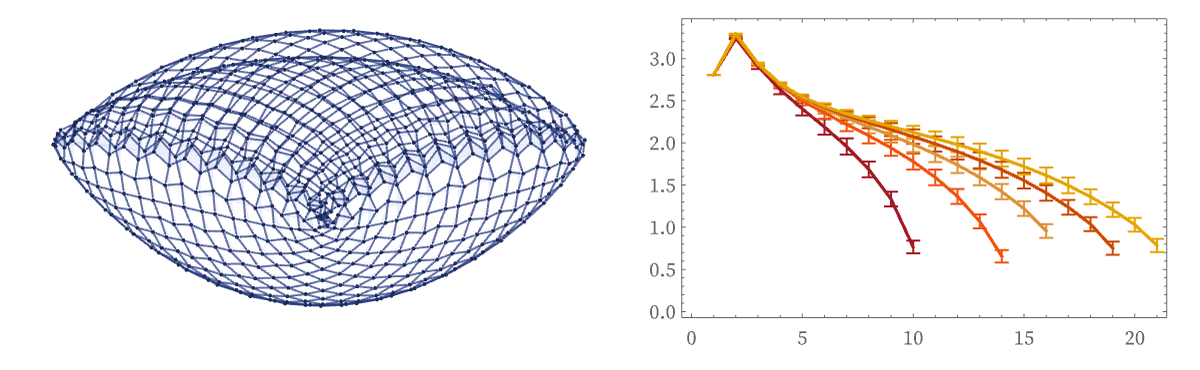
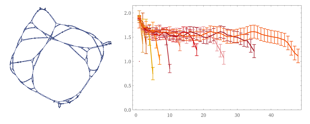
Now consider the sequence of “sphere” graphs:

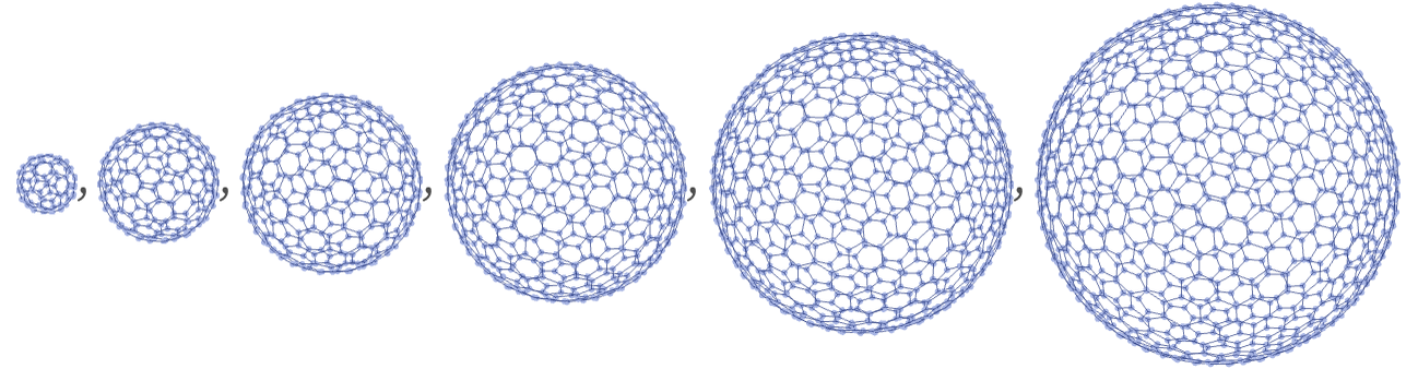
We can compute V_r for each of these graphs. Here are the log differences Δ(r) (the error bars come from the different neighborhoods associated with hexagonal and pentagonal “faces” in the graph):

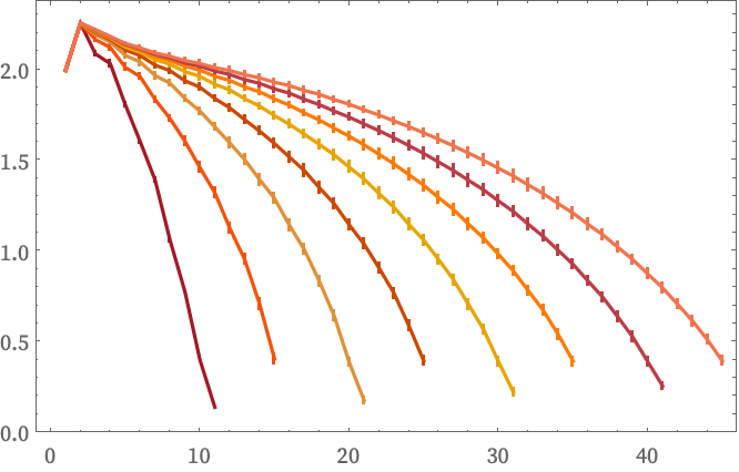
We immediately see the effect of curvature: even though in the limit the graphs effectively define 2D surfaces, the presence of curvature introduces a negative correction to pure r² growth in V_r. (Somewhat confusingly, there is only one scale defined for the kind of “pure sphere” graphs shown here, so they all have the same curvature, independent of size.)

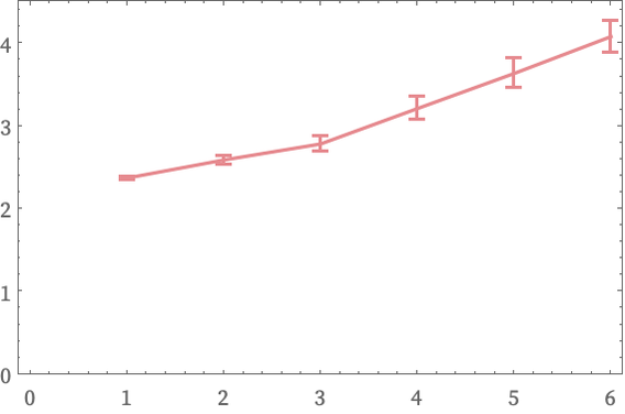
A torus, unlike a sphere, has no intrinsic surface curvature. So torus graphs of the form

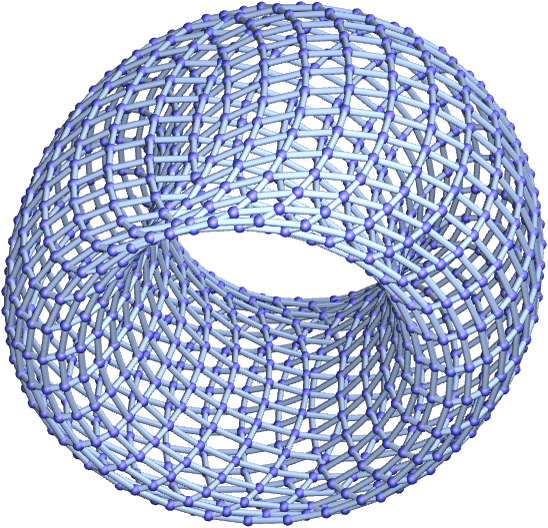
give flat log differences for V_r:

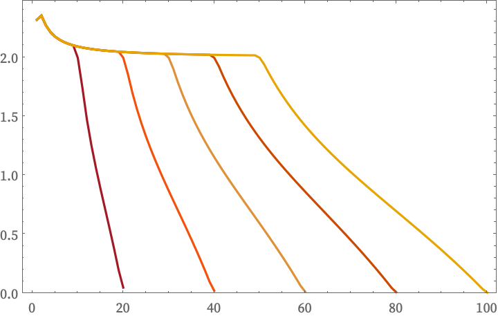
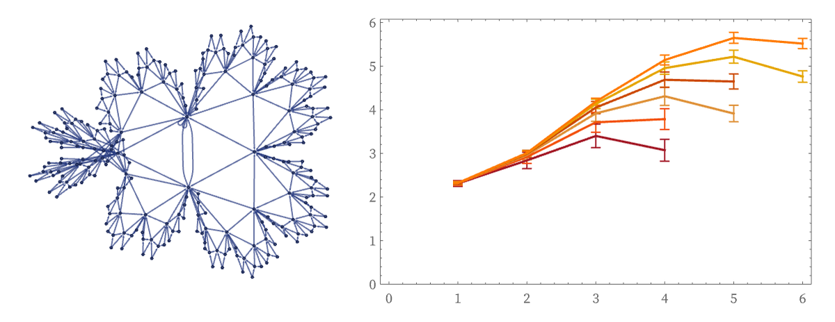
A graph based on a tiling in hyperbolic space

has negative curvature, so leads to a positive correction to V_r:

(One can imagine getting other examples by taking 3D objects and putting meshes on their surfaces. And indeed if the meshes are sufficiently faithful to the intrinsic geometry of the surfaces—say based on their geodesics—then the V_r(X) for the connectivity graphs of these meshes [28] will reflect the intrinsic curvatures of the surfaces. In practical computational geometry, though, meshes tend to be based on things like coordinate parametrizations, and so do not reflect intrinsic geometry.)

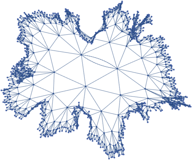
Many structures produced by our models exhibit curvature. There are cases of negative curvature:

As well as positive curvature:

The most obvious examples of nested structures have fractional dimension, but no curvature:

But even though it is not well characterized using ideas from traditional calculus, there is every reason to expect that the limits of our models can exhibit a combination of fractional dimension and curvature.

In general, though, there is no obvious constraint on the possible limiting form of V_r. Curvature can be thought of as associated with the O(r²) term in a Taylor expansion of V_r about r = 0, after factoring out r^d. But there is nothing to say that the leading behavior of V_r should match a form like r^d. In addition to exponentials like λ^r it could show an infinite collection of intermediate asymptotic scales, like 2^{r log(r)} or [29][30].