4.3 Geometry from Subdivision

The grids and surfaces that we saw above were all produced by rules that end up executing a laborious “knitting” process in which they add just a single relation at each step. But it is also possible to generate recognizable geometric forms more quickly—in effect by a process of repeated subdivision.

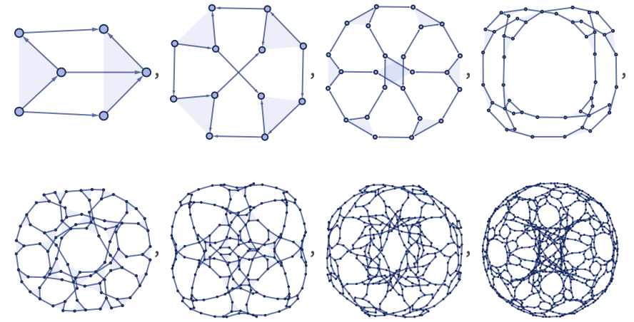
Consider the 2₃1₂  4₃4₂ rule:

RulePlot[ResourceFunction[ "WolframModel"][{{1, 2, 3}, {4, 5, 6}, {1, 4}} -> {{2, 7, 8}, {3, 9, 10}, {5, 11, 12}, {6, 13, 14}, {13, 8}, {7, 10}, {9, 12}, {11, 14}}]]

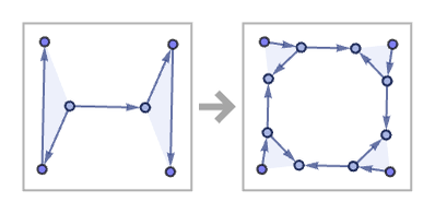
At each step, this rule doubles the number of relations—and quickly produces a structure with a definite emergent geometrical form:

ResourceFunction[ "WolframModel"][{{1, 2, 3}, {4, 5, 6}, {1, 4}} -> {{2, 7, 8}, {3, 9, 10}, {5, 11, 12}, {6, 13, 14}, {13, 8}, {7, 10}, {9, 12}, {11, 14}}, {{0, 0}, {0, 0}, {0, 0}, {0, 0, 0}, {0, 0, 0}}, 6, "StatesPlotsList"]

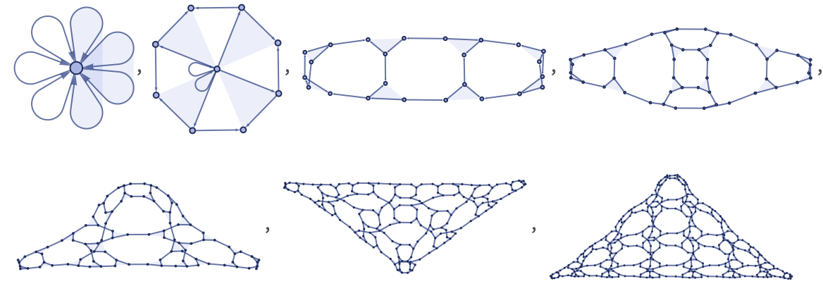
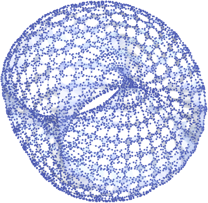
After 10 steps the rule has generated 2560 relations, in the following structure:

Visualized in 3D, this becomes:

ResourceFunction["GraphReconstructedSurface"][ ResourceFunction[ "WolframModel"][{{1, 2, 3}, {4, 5, 6}, {1, 4}} -> {{2, 7, 8}, {3, 9, 10}, {5, 11, 12}, {6, 13, 14}, {13, 8}, {7, 10}, {9, 12}, {11, 14}}, {{0, 0}, {0, 0}, {0, 0}, {0, 0, 0}, {0, 0, 0}}, 10, "FinalState"], 8]

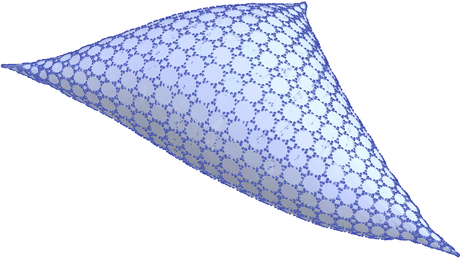
Once again, this corresponds to a smooth surface, but with 3 cusps. The surface is defined not by a simple triangular grid, but instead by an octagon-square (“truncated square”) tiling—that in this case becomes twice as fine at every step.

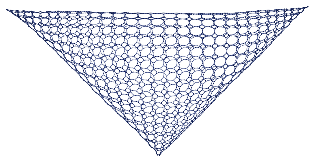
Changing the initial conditions can give a somewhat different structure:

ResourceFunction["WolframModelPlot"][#, ImageSize -> Tiny] & /@ ResourceFunction[ "WolframModel"][{{1, 2, 3}, {4, 5, 6}, {1, 4}} -> {{2, 7, 8}, {3, 9, 10}, {5, 11, 12}, {6, 13, 14}, {13, 8}, {7, 10}, {9, 12}, {11, 14}}, {{1, 2, 3}, {4, 5, 6}, {1, 4}, {2, 5}, {3, 6}}, 7, "StatesList"]

Visualized in 3D after 10 steps (and reconstructing less of the surface), this becomes:

ResourceFunction["GraphReconstructedSurface"][ ResourceFunction[ "WolframModel"][{{1, 2, 3}, {4, 5, 6}, {1, 4}} -> {{2, 7, 8}, {3, 9, 10}, {5, 11, 12}, {6, 13, 14}, {13, 8}, {7, 10}, {9, 12}, {11, 14}}, {{1, 2, 3}, {4, 5, 6}, {1, 4}, {2, 5}, {3, 6}}, 10, "FinalState"], 3]