4.4 Nested Patterns

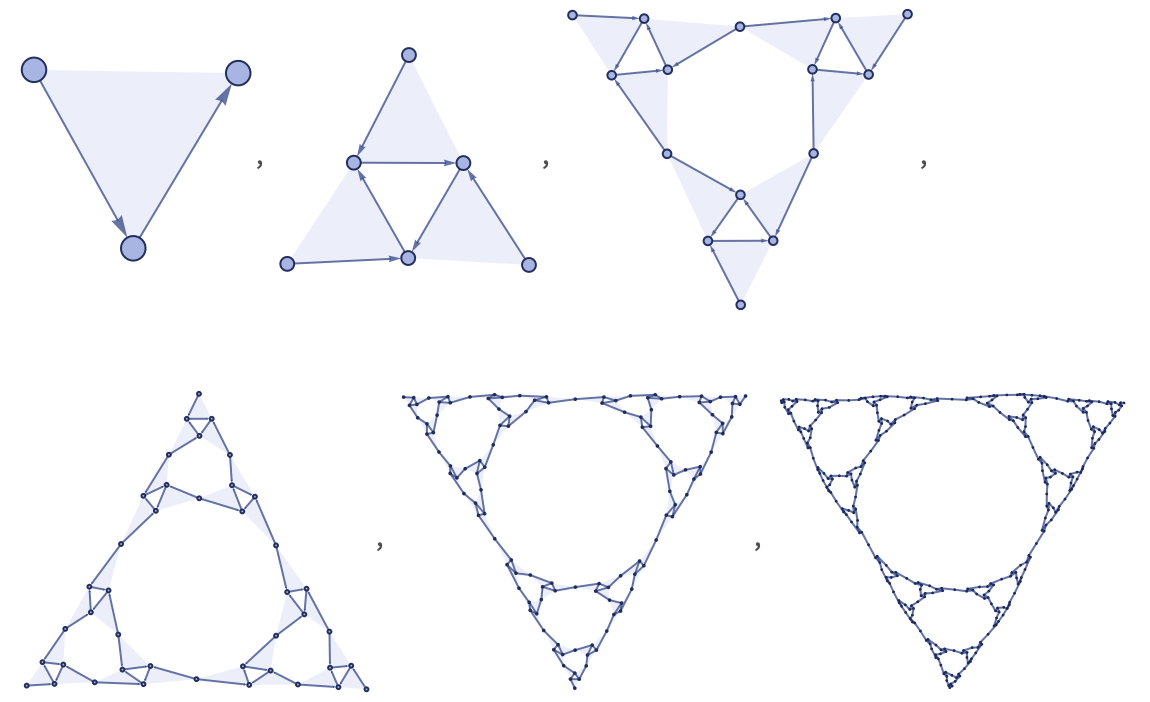
Consider the 1₃  3₃ rule:

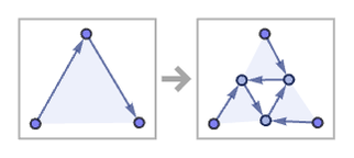
Starting from a single ternary relation with three distinct elements {{1,2,3}}, this gives a classic Sierpiński triangle structure:

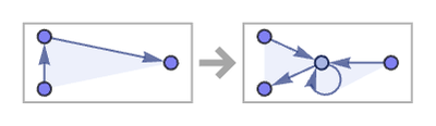
Starting instead from a ternary self-loop {{0,0,0}} one gets what amounts to a tetrahedron of Sierpiński triangles:

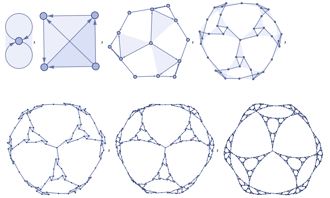
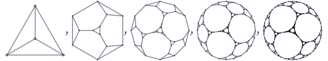
This is exactly the same as one would get by starting with a tetrahedron graph, and repeatedly replacing every trivalent vertex with a triangle of vertices [1:p509]:

In an ordinary Sierpiński triangle, the points on the edges have different neighborhoods from those in the interior. But in the structure shown here, all points have the same neighborhoods (so there is an isometry).

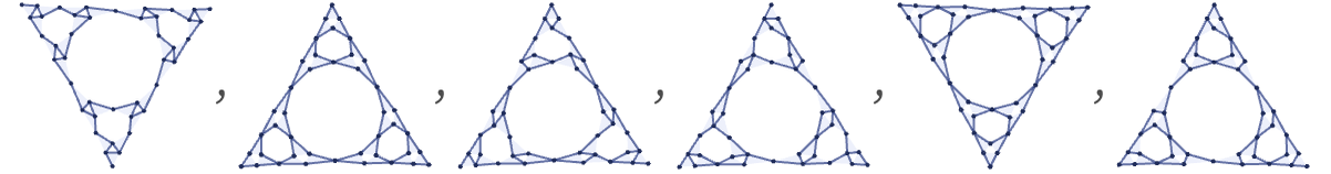
Many of the rules we have used have completely different behavior if the order of elements in their relations are changed. But in this case the limiting shape is always the same, regardless of ordering, as in these examples:

The rule we have discussed so far in this section in a sense directly implements the recursive construction of nested patterns [1:5.4]. But the formation of nested patterns is also a common feature of the limiting behavior of many rules that do not exhibit any such obvious construction.

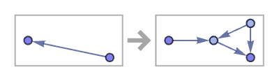
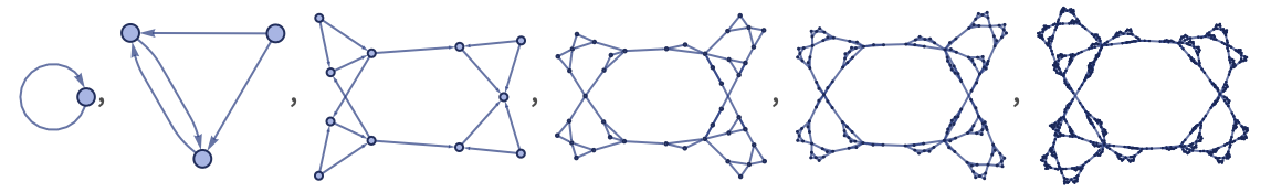
As an example, consider the 1₃  2₃ rule:

This rule effectively constructs a nested sequence of self-similar “segments”:

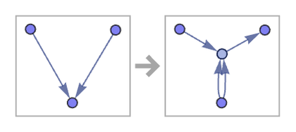
Similar behavior is seen in rules with binary relations, such as the 1₂  4₂ rule:

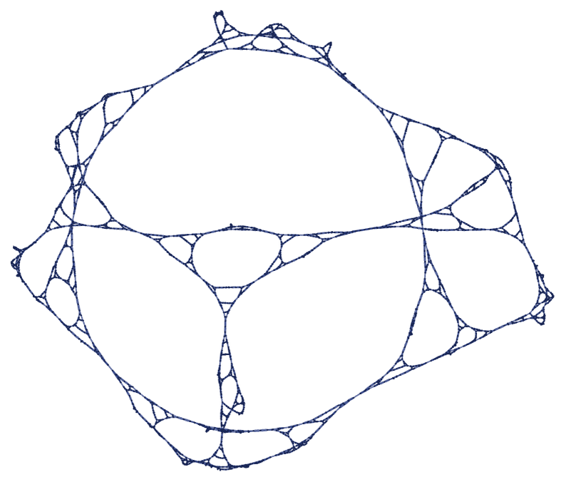
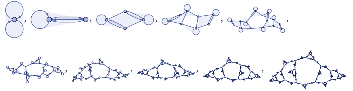
A clear “naturally occurring” Sierpiński pattern appears in the limiting behavior of the 2₂  4₂ rule:

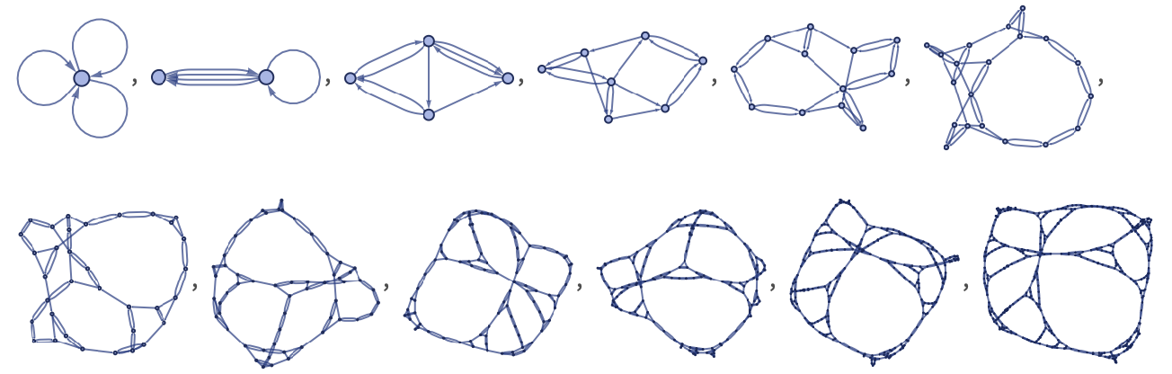
After 15 steps, the rule yields: