 download pdf
  ARXIV
ARXIV peer review
Most of our discussion so far has focused on how the structure of our models might correspond to the structure of our physical universe. But to make direct contact between our models and known physics, we need to fill in actual units and scales for the constructs in our models. In this section we give some indication of how this might work.
In our models, there is a fundamental unit of time (that we will call ![]() ) that represents the interval of time corresponding to a single updating event. This interval of time in a sense defines the scale for everything in our models.
) that represents the interval of time corresponding to a single updating event. This interval of time in a sense defines the scale for everything in our models.
Given ![]() , there is an elementary length
, there is an elementary length ![]() , determined by the speed of light c according to:
, determined by the speed of light c according to:
The elementary length defines the spatial separation of neighboring elements in the spatial hypergraph.
Another fundamental scale is the elementary energy ![]() : the contribution of a single causal edge to the energy of a system. The energy scale ultimately has both relativistic and quantum consequences. In general relativity, it relates to how much curvature a single causal edge can produce, and in quantum mechanics, it relates to how much change in angle in an edge in the multiway graph a single causal edge can produce.
: the contribution of a single causal edge to the energy of a system. The energy scale ultimately has both relativistic and quantum consequences. In general relativity, it relates to how much curvature a single causal edge can produce, and in quantum mechanics, it relates to how much change in angle in an edge in the multiway graph a single causal edge can produce.
The speed of light c determines the elementary length in ordinary space, specifying in effect how far one can go in a single event, or in a single elementary time. To fill in scales for our models, we also need to know the elementary length in branchial space—or in effect how far in state space one can go in a single event, or a single elementary time (or, in effect, how far apart in branchial space two members of a branch pair are). And it is an obvious supposition that somehow the scale for this must be related to ℏ.
An important point about scales is that there is no reason to think that elementary quantities measured with respect to our current system of units need be constant in the history of the universe. For example, if the universe effectively just splits every spatial graph edge in two, the number of elementary lengths in what we call 1 meter will double, and so the elementary length measured in meters will halve.
Given the structure of our models, there are two key relationships that determine scales. The first—corresponding to the Einstein equations—relates energy density to spacetime curvature, or, more specifically, gives the contribution of a single causal edge (with one elementary unit of energy) to the change of Vr and the corresponding Ricci curvature:
(Here we have dropped numerical factors, and G is the gravitational constant, which, we may note, is defined with its standard units only when the dimension of space d = 3.)
The second key relationship that determines scales comes from quantum mechanics. The most obvious assumption might be that quantum mechanics would imply that the elementary energy should be related to the elementary time by ![]() . And if this were the case, then our various elementary quantities would be equal to their corresponding Planck units [137], as obtained with G = c = ℏ = 1 (yielding elementary length ≈ 10–35 m, elementary time ≈ 10–43 s, etc.)
. And if this were the case, then our various elementary quantities would be equal to their corresponding Planck units [137], as obtained with G = c = ℏ = 1 (yielding elementary length ≈ 10–35 m, elementary time ≈ 10–43 s, etc.)
But the setup of our models suggests something different—and instead suggests a relationship that in effect also depends on the size of the multiway graph. In our models, when we make a measurement in a quantum system, we are at a complete quantum observation frame—or in effect aggregating across all the states in the multiway graph that exist in the current slice of the foliation that we have defined with our quantum frame.
There are many individual causal edges in the multiway causal graph, each associated with a certain elementary energy ![]() . But when we measure an energy, it will be the aggregate of contributions from all the individual causal edges that we have combined in our quantum frame.
. But when we measure an energy, it will be the aggregate of contributions from all the individual causal edges that we have combined in our quantum frame.
A single causal edge, associated with a single event which takes a single elementary time, has the effect of displacing a geodesic in the multiway graph by a certain unit distance in branchial space. (The result is a change of angle of the geodesic—with the formation of a single branch pair perhaps being considered to involve angle ![]() .)
.)
Standard quantum mechanics in effect defines ℏ through E = ℏ ω. But in this relationship E is a measured energy, not the energy associated with a single causal edge. And to convert between these we need to know in effect the number of states in the branchial graph associated with our quantum frame, or the number of nodes in our current slice through the multiway system. We will call this number Ξ.
And finally now we can give a relation between elementary energy and elementary time:
In effect, ℏ sets a scale for measured energies, but ℏ/Ξ sets a scale for energies of individual causal edges in the multiway causal graph.
This is now sufficient to determine our elementary units. The elementary length is given in dimension d = 3 by
where lP, tP, EP are the Planck length, time and energy.
To go further, however, we must estimate Ξ. Ultimately, Ξ is determined by the actual evolution of the multiway system for a particular rule, together with whatever foliation and other features define the way we describe our experience of the universe. As a simple model, we might then characterize what we observe as being “generational states” in the evolution of a multiway system, as we discussed in 5.21.
But now we can use what we have seen in studying actual multiway systems, and assume that in one generational step of at least a causal invariant rule each generational state generates on average some number κ of new states, where κ is related to the number of new elements produced by a single updating event. In a generation of evolution, therefore, the total number of states in the multiway system will be multiplied by a factor κ.
But to relate this to observed quantities, we must ask what time an observer would perceive has elapsed in one generational step of evolution. From our discussion above, we expect that the typical time an observer will be able to coherently maintain the impression of a definite “classical-like” state will be roughly the elementary time ![]() multiplied by the number of nodes in the branchlike hypersurface. The number of nodes will change as the multiway graph grows. But in the current universe we have defined it to be Ξ.
multiplied by the number of nodes in the branchlike hypersurface. The number of nodes will change as the multiway graph grows. But in the current universe we have defined it to be Ξ.
Thus we have the relation
where tH is the current age of the universe, and for this estimate we have ignored the change of generation time at different points in the evolution of the multiway system.
Substituting our previous result for ![]() we then get:
we then get:
There is a rough upper limit on κ from the signature for the underlying rule, or effectively the ratio in the size of the hypergraphs between the right and left-hand sides of a rule. (For most of the rules we have discussed here, for example, κ ≲ 2.) The lower limit on κ is related to the “efficiency” of causal invariance in the underlying rule, or, in effect, how long it takes branch pairs to resolve relative to how fast new ones are created. But inevitably κ > 1.
Given the transcendental equation
we can solve for Ξ to get
where W is the product log function [138] that solves w ew = z. But for large σ log(κ) (and we imagine that σ ≈ 1061), we have the asymptotic result [30]:
Plotting the actual estimate for Ξ as a function of κ we get the almost identical result:
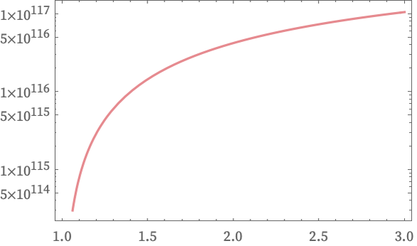
If κ = 1, then we would have Ξ = 1, and for κ extremely close to 1, Ξ ≈ 1 + σ (κ – 1) + ... But even for κ = 1.01 we already have Ξ ≈ 10112, while for κ = 1.1 we have Ξ ≈ 10115, for κ = 2 we have Ξ ≈ 4 × 10116 and for κ = 10 we have Ξ ≈ 5 × 10117.
To get an accurate value for κ we would have to know the underlying rule and the statistics of the multiway system it generates. But particularly at the level of the estimates we are giving, our results are quite insensitive to the value of κ, and we will assume simply:
In other words, for the universe today, we are assuming that the number of distinct instantaneous complete quantum states of the universe being represented by the multiway system (and thus appearing in the branchial graph) is about 10116.
But now we can estimate other quantities:
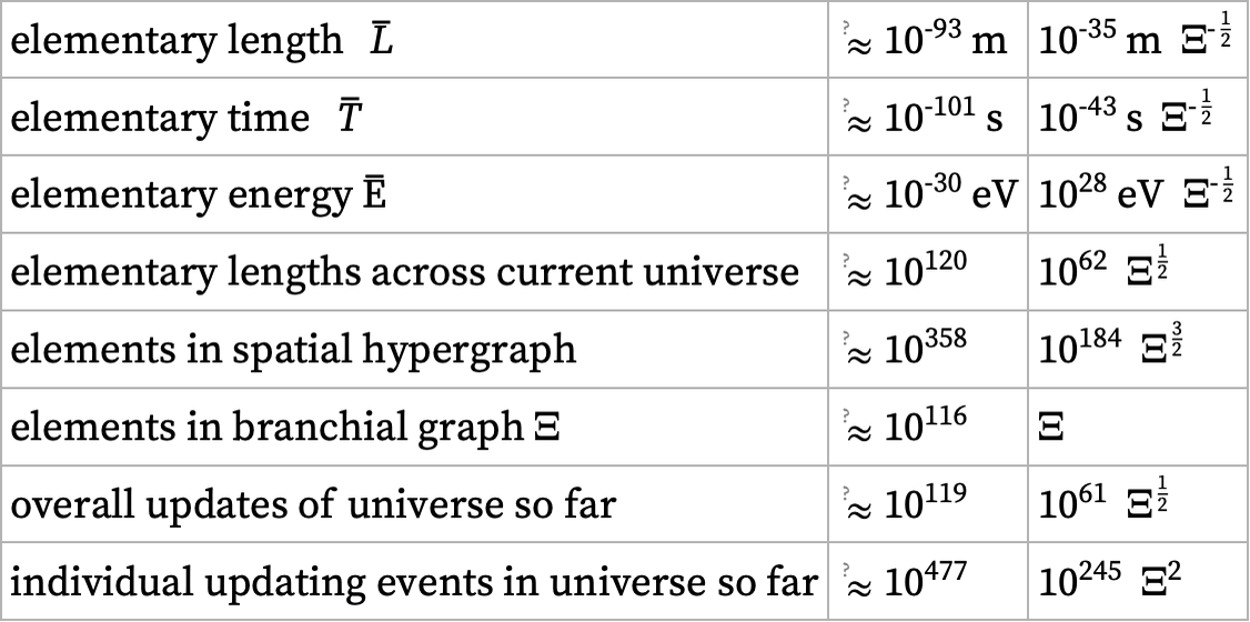
The fact that our estimate for the elementary length ![]() is considerably smaller than the Planck length indicates that our models suggest that space may be more closely approximated by a continuum than one might expect.
is considerably smaller than the Planck length indicates that our models suggest that space may be more closely approximated by a continuum than one might expect.
The fact that the elementary energy ![]() is much smaller than the surprisingly macroscopic Planck energy (≈ 1019 GeV ≈ 2 GJ, or roughly the energy of a lightning bolt) is a reflection of the fact the Planck energy is related to measurable energy, not the individual energy associated with an updating event in the multiway causal graph.
is much smaller than the surprisingly macroscopic Planck energy (≈ 1019 GeV ≈ 2 GJ, or roughly the energy of a lightning bolt) is a reflection of the fact the Planck energy is related to measurable energy, not the individual energy associated with an updating event in the multiway causal graph.
Given the estimates above, we can use the rest mass of the electron to make some additional very rough estimates—subject to many assumptions—about the possible structure of the electron:
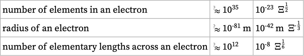
In quantum electrodynamics and other current physics, electrons are assumed to have zero intrinsic size. Experiments suggest that any intrinsic size must be less than about 10–22 m [139][140]—nearly 1060 times our estimate.
Even despite the comparatively large number of elements suggested to be within an electron, it is notable that the total number of elements in the spatial hypergraph is estimated to be more than 10200 times the number of elements in all known particles of matter in the universe—suggesting that in a sense most of the “computational effort” in the universe is expended on the creation of space rather than on the dynamics of matter as we know it.
The structure of our models implies that not only length and time but also energy and mass must ultimately be quantized. Our estimates indicate that the mass of the electron is > 1036 times the quantized unit of mass—far too large to expect to see “numerological relations” between particle masses.
But with our model of particles as localized structures in the spatial hypergraph, there seems no reason to think that structures much smaller than the electron might not exist—corresponding to particles with masses much smaller than the electron.
Such “oligon” particles involving comparatively few hypergraph elements could have masses that are fairly small multiples of 10–30 eV. One can expect that their cross-sections for interaction will be extremely small, causing them to drop out of thermal equilibrium extremely early in the history of the universe (e.g. [141][142]), and potentially leading to large numbers of cold, relic oligons in the current universe—making it possible that oligons could play a role in dark matter. (Relic oligons would behave as a more-or-less-perfect ideal gas; current data indicates only that particles constituting dark matter probably have masses ≳ 10–22 eV [143].)
As we discussed in the previous subsection, the structure of our models—and specifically the multiway causal graph—indicates that just as the speed of light c determines the maximum spacelike speed (or the maximum rate at which an observer can sample new parts of the spatial hypergraph), there should also be a maximum branchlike speed that we call ζ that determines the maximum rate at which an observer can sample new parts of the branchial graph, or, in effect, the maximum speed at which an observer can become entangled with new “quantum degrees of freedom” or new “quantum information”.
Based on our estimates above, we can now give an estimate for the maximum entanglement speed. We could quote it in terms of the rate of sampling quantum states (or branches in the multiway system)
but in connecting to observable features of the universe, it seems better to quote it in terms of the energy associated with edges in the causal graph, in which case the result based on our estimates is:
This seems large compared to typical astrophysical processes, but one could imagine it being relevant for example in mergers of galactic black holes.