 download pdf
  ARXIV
ARXIV peer review
We have discussed causal invariance in terms of path independence in multiway systems. But we can also explore it in terms of specific evolution histories for the underlying substitution system. Consider the rule {BA AB}. Here is a representation of one way it can act on a particular initial string:
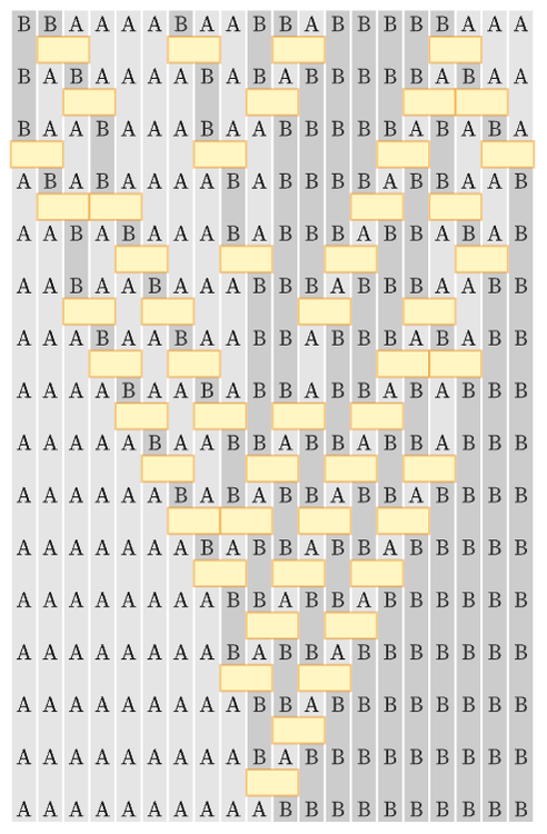
In a multiway system, each path represents a particular sequence of updates that occur one after another. But here in showing the action of {BA AB} we are choosing to draw several updates on the same row. If we want, we can think of these updates as being done in sequence, but since they are all independent, it is consistent to show them as we do.
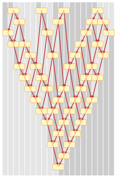
If we annotate the picture by showing causal connections between updates, we see the causal graph for the evolution—and we see that the updates we have drawn on the same row are indeed independent: they are not connected in the causal graph:
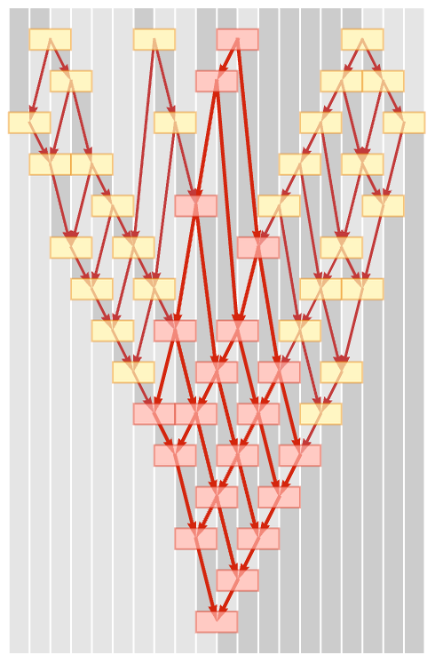
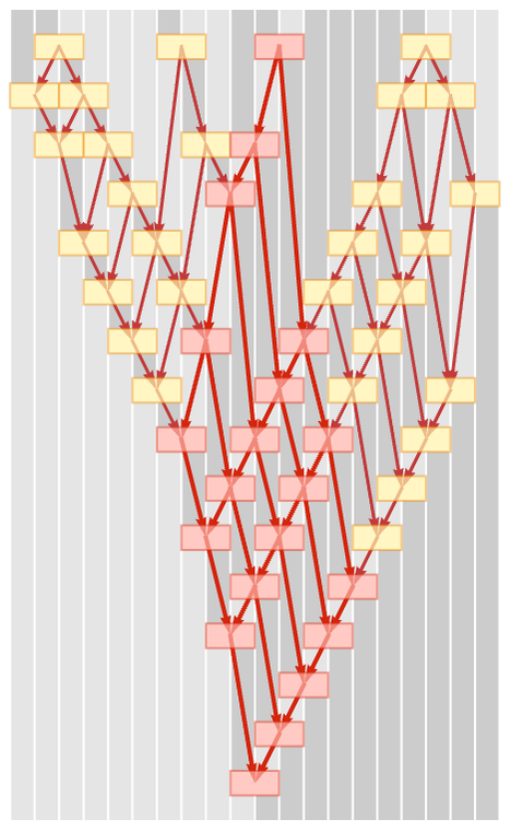
The picture above in effect uses a particular updating order. The pictures below show three possible random choices of updating orders. In each case, the final result of the evolution is the same. The intermediate steps, however, are different. But because our rule is causal invariant, the causal graph of causal relationships always has exactly the same form:
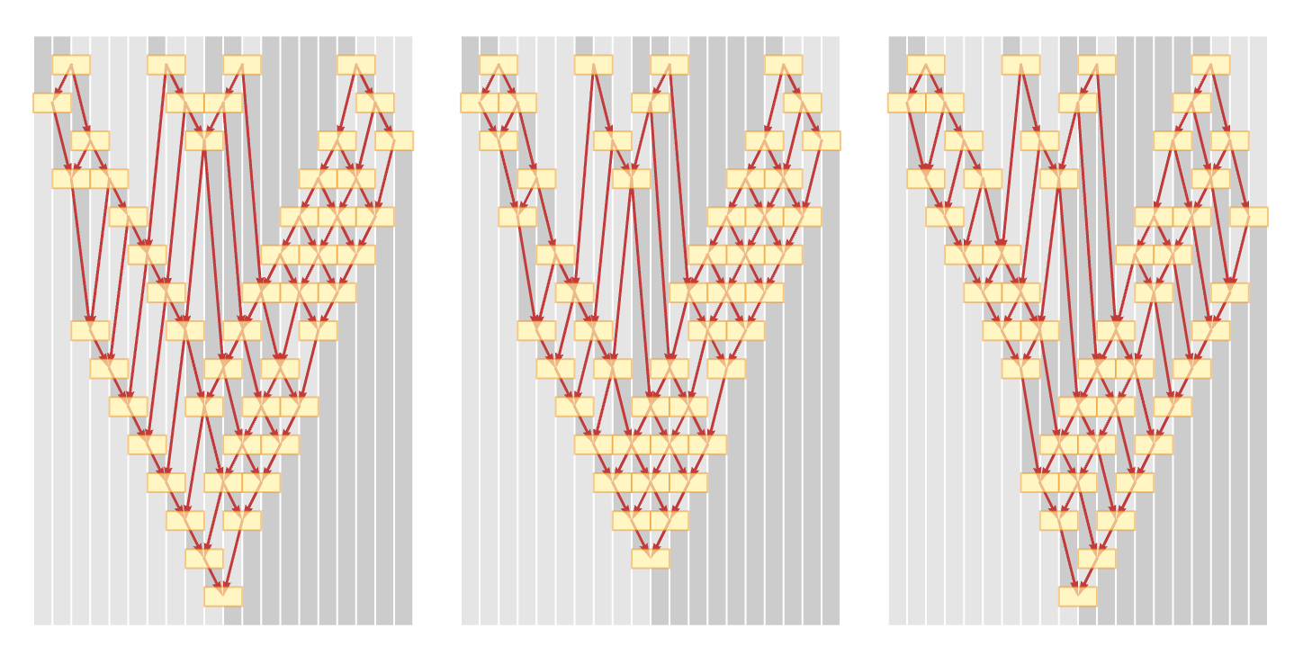
In picking updating orders there is always one constraint: no update can happen until the input for it is ready. In other words, if the input for update V comes from the output of update U, then U must already have happened before V can be done. But so long as this constraint is satisfied, we can pick whatever order of updates we want (cf. [1:9.10]).
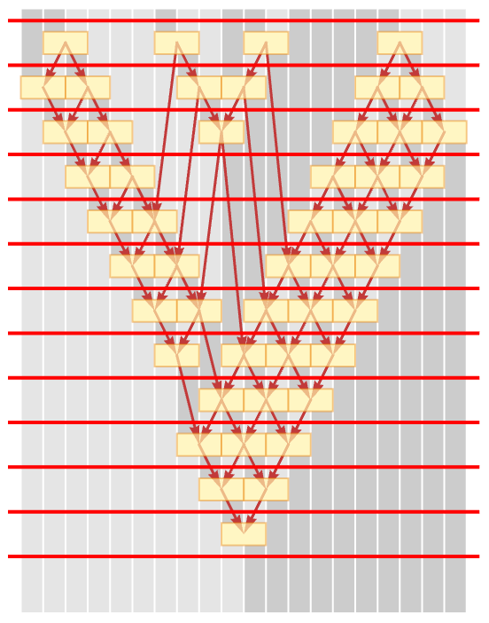
It is sometimes convenient, however, to think in terms of “complete steps of evolution” in which all updates that could yet be done have been done. And for the particular rule we are currently discussing, we can readily do this, separating each “complete step” in the pictures below with a red line:
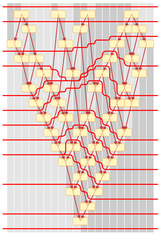
Where the red lines go depends on the update order we choose. But because of causal invariance it is always possible to draw them to delineate steps in which a collection of independent updates occur.
Each choice of how to assign updates to steps in effect defines a foliation of the evolution. We will call foliations in which the updates at each step are causally independent “causal foliations”. Such causal foliations are in effect orthogonal to the connections defined by the causal graph. (In physics, the analogy is that the causal foliations are like foliations of spacetime defined by a sequence of spacelike hypersurfaces, with connections in the causal graph being timelike.)
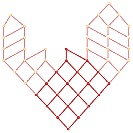
The fact that our underlying substitutions (in this case just BA AB) involve neighboring elements implies a certain locality to the process of evolution. The consequence of this is that we can meaningfully discuss the “spatial” spreading of causal effects. For example, consider tracing the causal connections from one event in our system:
In effect there is a cone (here just two-dimensional) of elements in the system that can be affected. We will call this the causal cone for the evolution. (In physics, the analogy is a light cone.) If we pick a different updating order, the causal cone is distorted. But viewed in terms of the causal foliations, it is exactly the same:
This is the result purely in terms of the causal graph:
Now let us turn things around. Imagine we have a causal graph. Then we can ask how it relates to an actual sequence of states generated by a particular path of evolution. The pictures below show how we can arrange a causal graph so that its nodes—corresponding to events—appear at positions down the page that correspond to a particular causal foliation and thus a particular path of evolution:
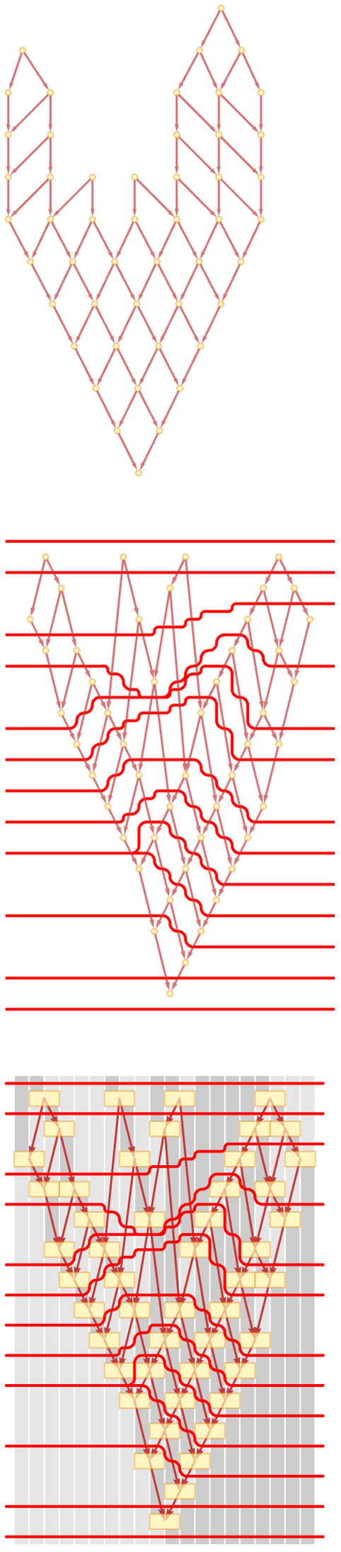
It is worth noticing that at least for the rule we are using here the intrinsic structure of the causal graph defines a convenient foliation in which successive events are simply arranged in layers:
The rule BA AB that we are using has many simplifying features. But the concepts of causal foliations and causal cones are general, and will be important in much of what follows.
As it happens, we have already implicitly seen both ideas. The “standard updating order” for our main models defines a foliation (similar, in fact, to the last one we showed here, in which in some sense “as much gets done as possible” at each step)—though the foliation is only a causal one if the rule used is causal invariant.
In addition, in 4.14 we discussed how the effect of a small change in the state in one of our models can spread on subsequent steps, and this is just like the causal cone we are discussing here.