download pdf
  ARXIV
ARXIV peer review
One might think that all rules would work like the one we just studied, and would give different causal graphs depending on what specific path of evolution one chose, or what updating scheme one used. But a crucial fact that will be central to the potential application of our models to physics is this is not the case.
Instead, whenever a rule is causal invariant, it does not produce many different causal graphs. Instead, whatever specific path of evolution one choses, the rule always yields an exactly equivalent causal graph.
The rule we just studied is not causal invariant. But consider instead the simple causal invariant rule {BA AB} evolving from the state BBBAA:
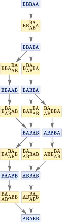
Adding in causal relationships this becomes:
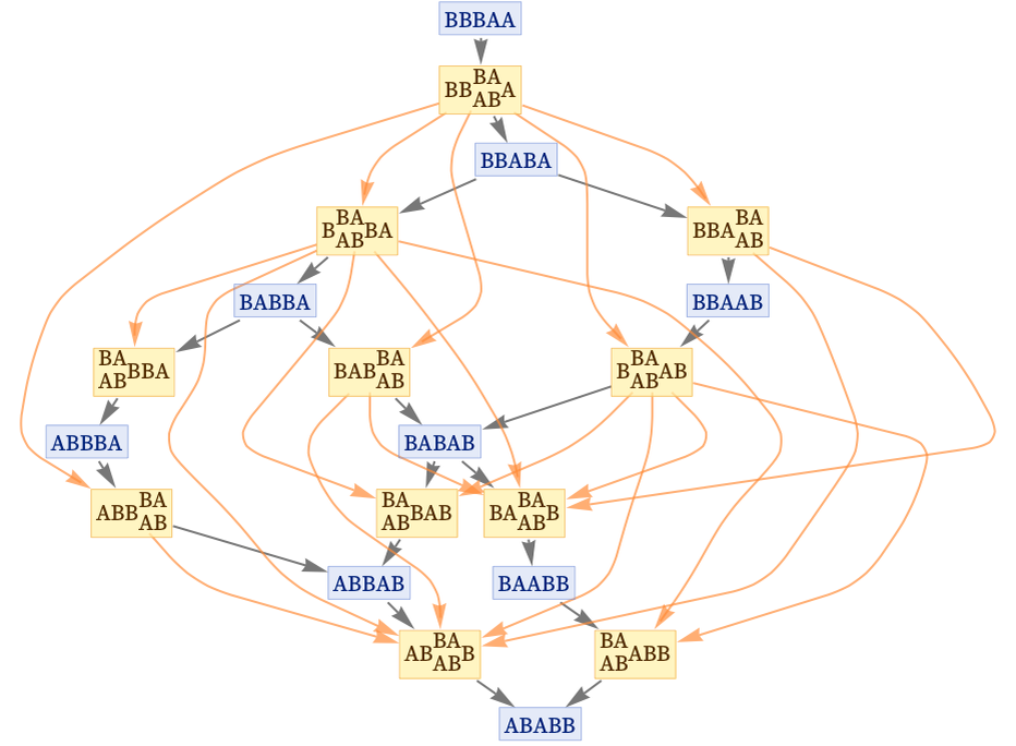
The corresponding multiway causal graph is:
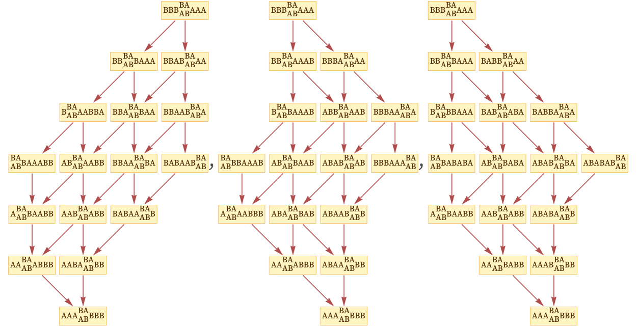
But now consider the individual causal graphs, corresponding to different possible paths of evolution. From the multiway causal graph we can extract all of these, and the result is:
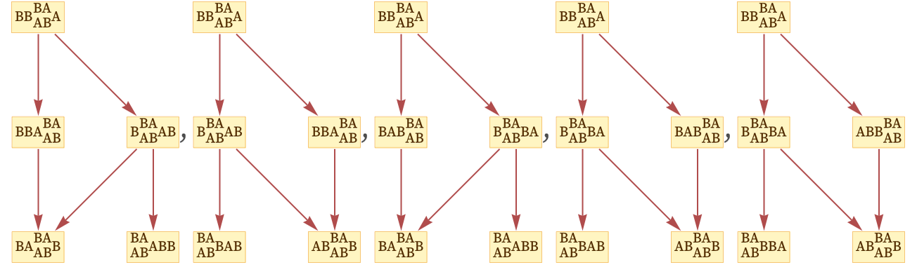
There are five different cases. But the remarkable fact is that they all correspond to isomorphic graphs. In other words. even though the specific sequence of states that the system visits is different in each case, the network of causal relationships is always exactly the same, regardless of what path is followed.
And this is a general feature of any causal invariant system. The underlying evolution rules for the system may allow many different paths of evolution—and many different sequences of states. But when the rules for the system are causal invariant, it means that the network of relationships between updating events is always the same. Depending on the particular order in which updates are done, one can see different paths of evolution; but if one looks only at event updates and their relationships, there is just one thing the system does.
Here is a slightly larger example for the rule {BA AB} starting from BBBBAAAA. In each case a different random updating order is used, leading to a different sequence of states. But the final causal graphs representing the causal relationships between events are exactly the same: