5.21 Generational Evolution

Systems like cellular automata always update every element at every step in their evolution. But in string substitution systems (as well as in our hypergraph-based models), the presence of overlaps between possible updating events typically means that there is no single, consistent way to do this kind of parallel updating. Nevertheless, in studying our models in earlier sections, we often used “steps” of evolution in which we updated as many elements as we consistently could. And we can also apply this kind of “generation-based” updating to string substitution systems.

Consider the rule:

We can construct the multiway graph for this rule by considering how one state is produced from another by a single updating event, corresponding to a single application of one of the transformations in the rule:

But we can also consider producing a “generational multiway graph” in which we do as many non-overlapping updates as possible on any given string. For this particular rule, doing this is straightforward, since every A and every B in the string can be transformed separately.

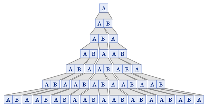
But the result is now a radically simplified multiway graph, in which there is just a single path of evolution:

The “generational steps” here involve an increasing number of update events, as we can see from this rendering of the evolution:

All the states obtained at generational steps do appear somewhere in the full multiway graph, but the full graph also contains many additional states—that, among other things, can be thought of as representing all possible intermediate stages of generational steps:

For a rule like

the generational steps

correspond to a particularly simple trajectory through the full multiway graph:

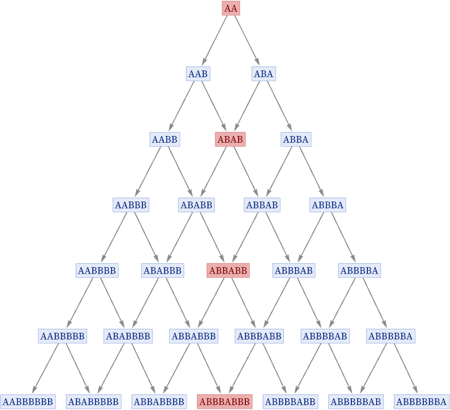
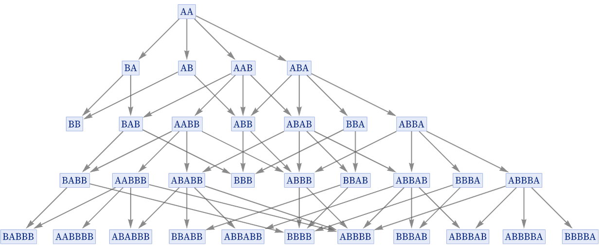
It is not always the case that the generational multiway graph involves just a single path. Consider the rule:

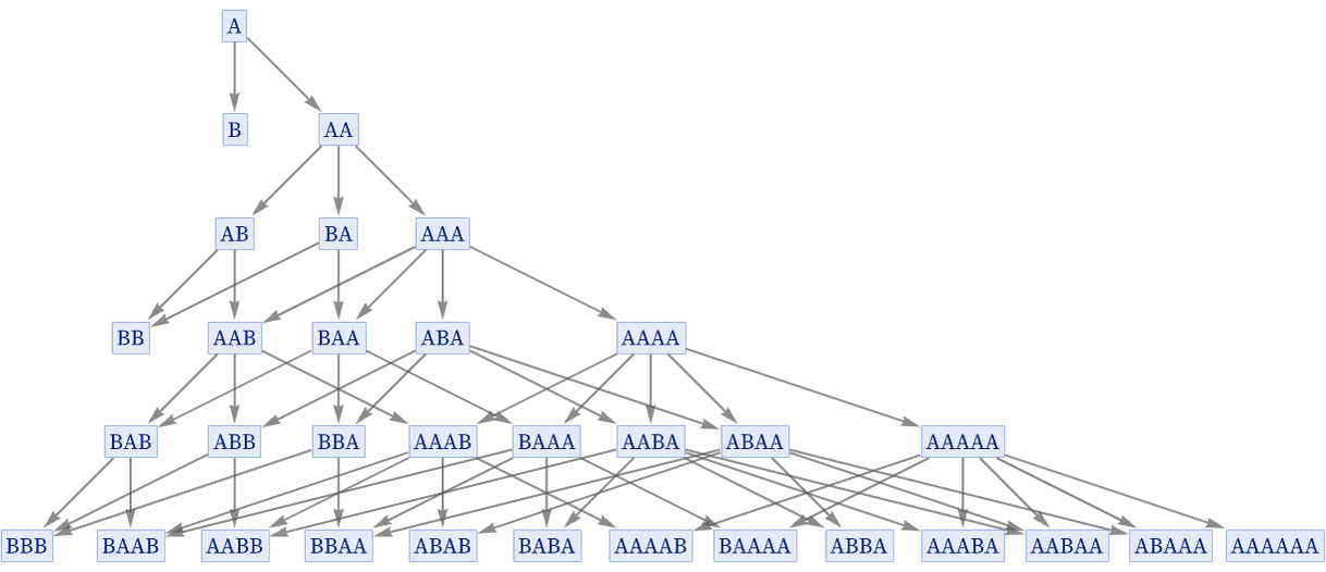
The ordinary multiway graph for this rule starting from AA is:

And the generational multiway graph is now:

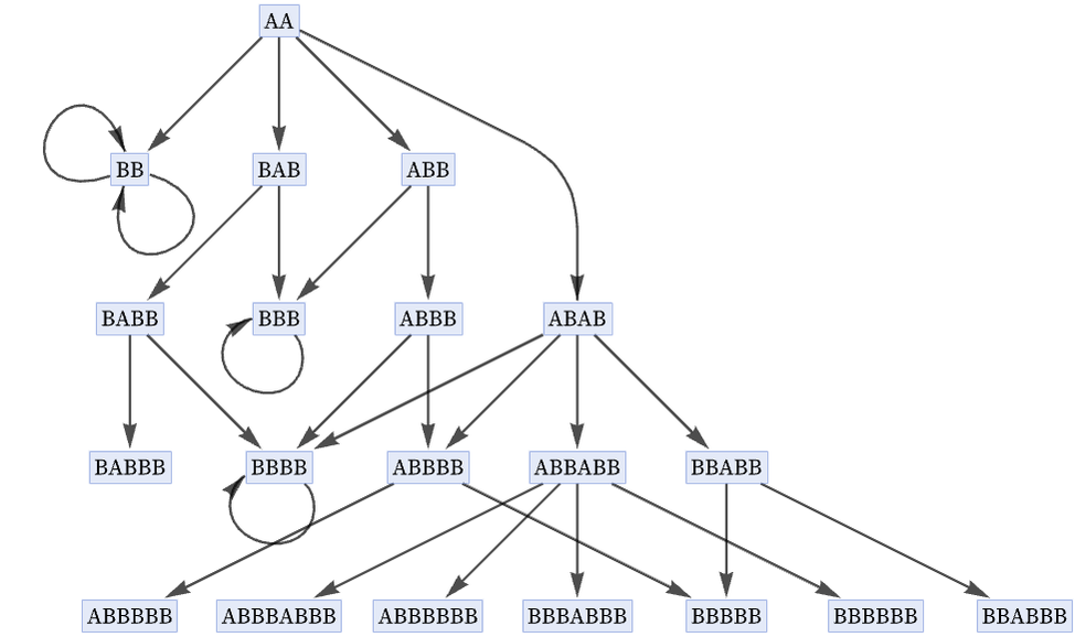
The generational multiway graph is always in a sense a compression of the full multiway graph. And one way to think of it is as being derived from the full multiway graph by combining sequences of edges when they correspond to updating events that do not overlap on the string.

But there is also another view of generational evolution. Consider a branchial graph from the full multiway graph above (this branchial graph is derived from the layered foliation shown):

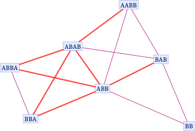
The branch pairs in this branchial graph (shown as adjacent nodes) can be thought of as being of two kinds. The first are produced by applying different rules to a single part of a string (e.g. ABA  {ABBA, BBA}). And the second (highlighted in the graph above) by applying rules to different parts of a string (e.g. ABA  {ABBA, ABAB}).

In the full multiway graph, no distinction is made between these two kinds of branch pairs, and the graph includes both of them. But in a generational multiway system, strings in the second kind of branch pairs can be combined.

And indeed this provides another way to construct a generational multiway system: look at branchial graphs and take pairs of strings corresponding to “spatially” disjoint updating events, and then knit these together to form generational steps. And if there is only one way to do this for each branchial graph, one will get a single path of generational evolution. But if there are multiple ways, then the generational multiway graph will be more complicated.

For the rule

that we discussed above, the sequence of branchial graphs is

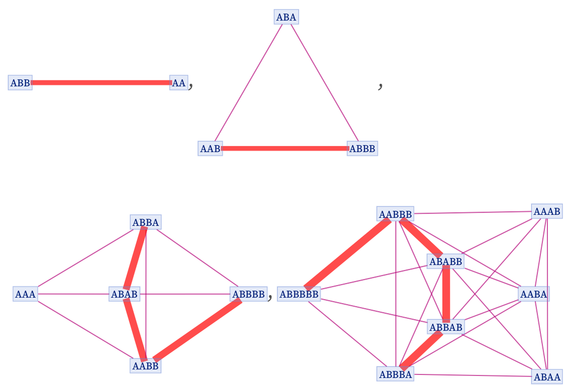
and it is readily possible to assemble “string fragments” (such as those highlighted) to produce the states at successive generational steps:

The branchial graphs are determined by the foliation of the multiway graph that one uses. But given a foliation, one can then assemble strings corresponding to generational steps using the procedure above.

There is always an alternative, however: instead of combining strings from a branchial graph to produce the state for a generational step, one can always in a sense just wait, and eventually the full multiway system will have done the necessary sequence of updates to produce the complete state for the generational step.

Whenever there are no possible overlaps in the application of rules, the generational multiway graph must always yield a single path of history. But there is also another feature of such rules: they are guaranteed to be causal invariant. There are, however, plenty of rules that are causal invariant even though they allow overlaps—in a sense because their right-hand sides also appropriately agree. And for such rules, the generational multiway graph may have multiple paths of history.

A simple example is the rule:

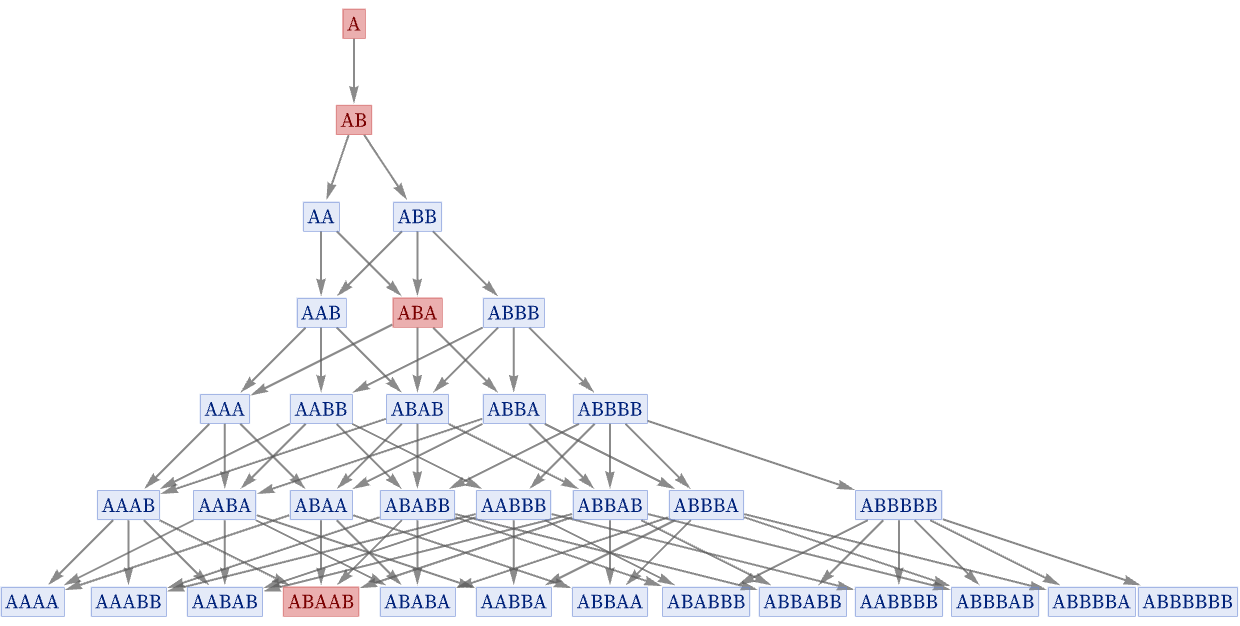
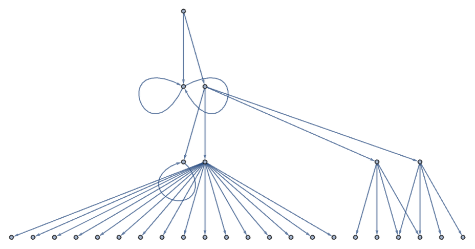
This rule is causal invariant, and starting from A yields the full multiway graph:

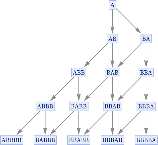
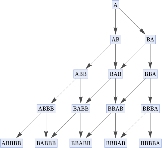
Its generational multiway graph is actually identical in this case—because all the rule ever does is to apply one transformation or the other to the single A that appears:

Starting from AA, however, the rule yields the full multiway graph

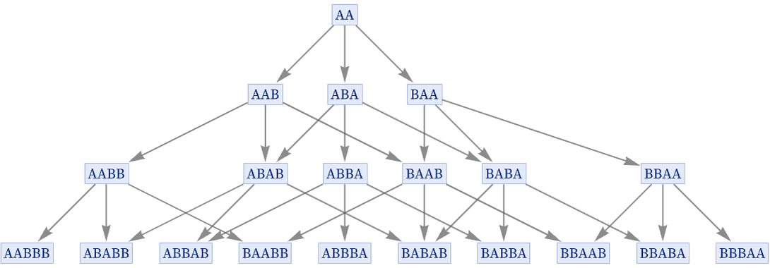
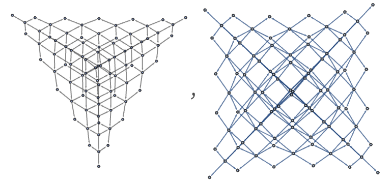
and the generational multiway graph:

In an alternative rendering, these graphs after a few more steps become, respectively:

Note that in both cases, the number of states reached after t steps grows like t² (in the first case it is ; in the second case exactly t²).

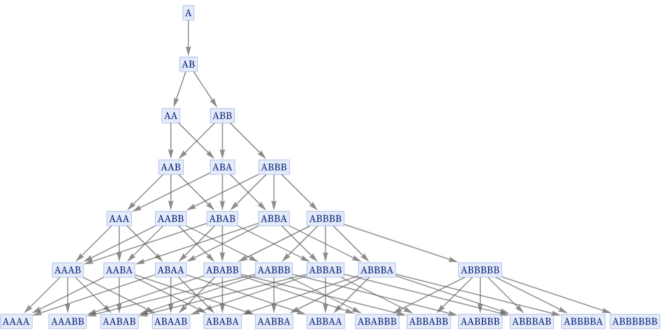
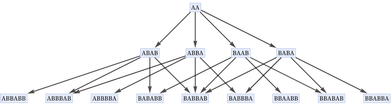
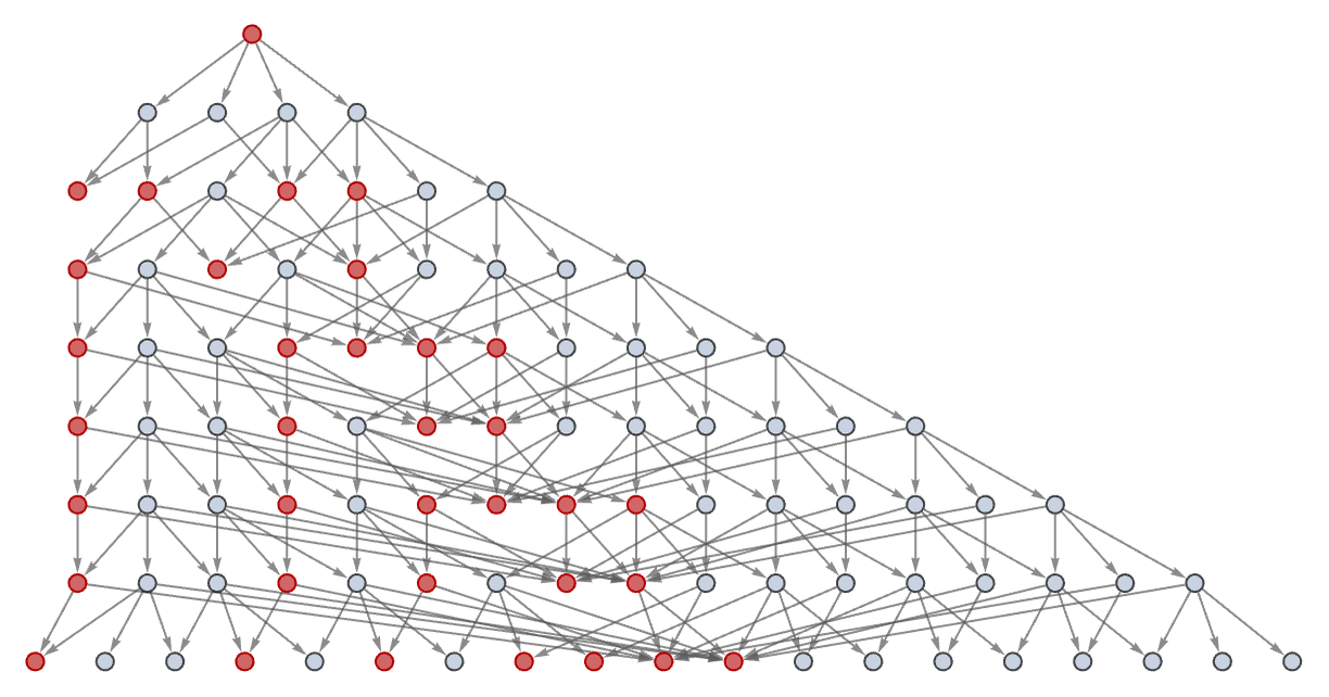
In the case of a rule like

the presence of many potential overlaps in where updates can be applied makes many of the possible states in the full multiway graph also appear in the generational multiway graph (in the limit about 64% of all possible states are generational results):

Generational multiway graphs share many features with full multiway graphs. For example, generational multiway graphs can also show causal invariance—and indeed unless strings grow too fast, any deviation from causal invariance must also appear in the generational multiway graph.

The basic construction of ordinary multiway graphs ensures that the number of states M_t after t steps can grow at most exponentially with t. In a generational multiway graph, there can be faster growth.

Consider for example the rule:

Its full multiway graph grows in a Fibonacci sequence ≈ϕ^t:

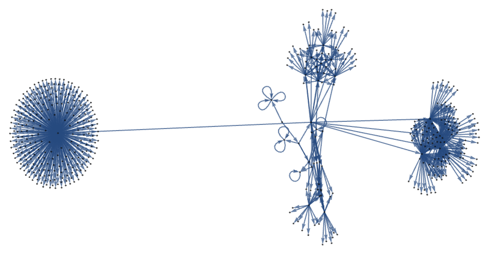
But its generational multiway graph grows much faster. After 3 generational steps it has the form

while after 4 steps (in a different rendering) it is:

The number of states reached in successive steps is:

Although there is a distribution of lengths for the strings, say, at steps 4 and 5

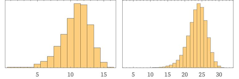
the fact that the maximum string length at generational step t is 2^t–1—combined with the lack of causal invariance for this rule—allows for double exponential growth in the number of possible states with generational steps. In fact, with this particular rule, by step t almost all sequences of up to 2^t–1 Bs and AAs have appeared (the missing fractions on steps 3, 4, 5 are 0.13, 0.078, 0.017) so at step t the total number of states approaches