 download pdf
  ARXIV
ARXIV peer review
In any causal invariant rule, all branch pairs that are generated must eventually resolve. But by looking at how many branch pairs are resolved—and unresolved—at each step, we can get a sense of “how far” a rule is from causal invariance.
Consider the causal invariant rule:
With this rule, all branch pairs resolve in one step
and the total number of branch pairs that have already resolved on successive steps is (roughly 2t):
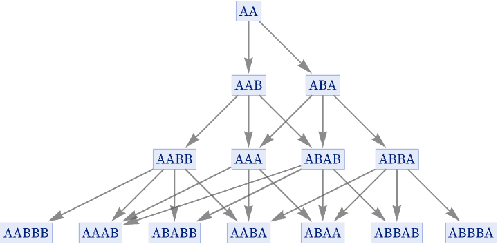
But now consider the slightly different—and non-causal-invariant—rule:
The number of resolved branch pairs goes up on successive steps—in this case quadratically:
But now there is a “residue” of new unresolved branch pairs at each step that reflect the lack of causal invariance:
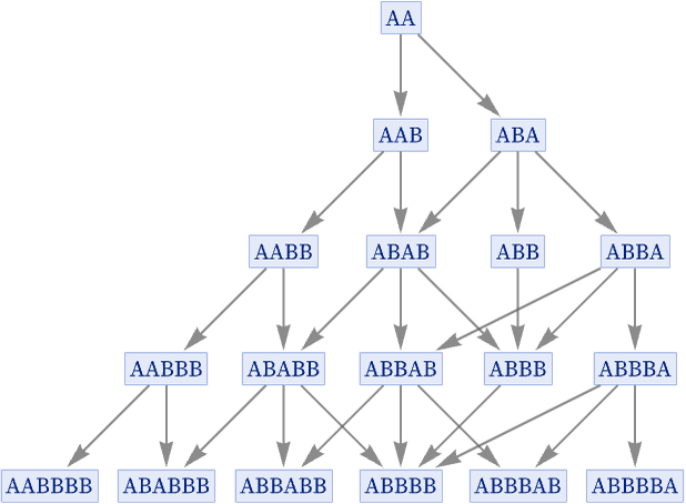
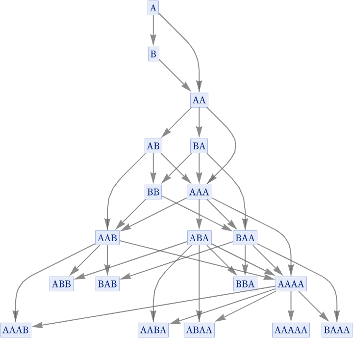
There are other rules in which the deviation from causal invariance is in a sense larger. Consider the rule:
The multiway graph for this rule shows various “dead ends”
and now the number of resolved branch pairs is
while the number of unresolved ones grows at a similar rate:
When a system is not causal invariant, what it means is that in a sense the system can reach states from which it cannot ever “get back” to other states. But this suggests that by extending the rules for the system, one might be able to make it causal invariant.
Consider the rule
with multiway graph:
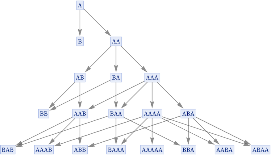
With this rule, the branch pair {B, AA} never resolves. But now let us just extend the rule by adding B AA:
The multiway graph becomes
and the rule is now causal invariant.
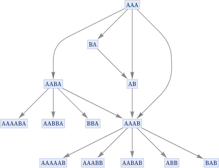
In general, given a rule that is not causal invariant, we can consider extending it by including transformations that relate strings in branch pairs that do not resolve. For the rule
discussed above it turns out that the minimal additions to achieve causal invariance are:
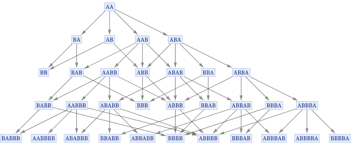
Having added these transformations, the multiway graph now begins:
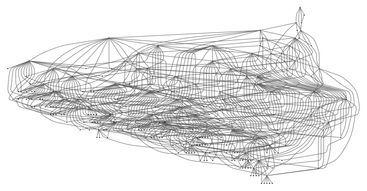
After more steps, the multiway graph is:
This kind of “completion” procedure of adding “relations” in order to achieve what amounts to causal invariance is familiar in automated theorem proving [82] and related areas [60]. For our purposes we can think of it as a kind of “coarse graining” of our systems, in which the additional rules in effect define equivalences between states that would otherwise be distinct.
If a particular multiway graph terminates after a finite number of steps, then it is always possible to add enough completion rules to the system to ensure causal invariance [63][64]. But if the multiway graph grows without bound, this may not be possible. Sometimes one may succeed in adding enough completions to achieve causal invariance for a certain number of steps, only to have it fail after more steps. And in general, like determining whether branch pairs will resolve, there is ultimately no upper bound on how long one may have to wait, making the problem of completion ultimately formally undecidable [83].
But if (as is often the case) one only has to add a small number of completion rules to make a system causal invariant, then one can take this to mean that the system is not far from causal invariance, so that it is likely that many of the large-scale properties of the completion of the system will be shared by the system itself.