5.1 String Substitution Systems

The basic concept of our models is to define rules for updating collections of relations. But for a particular collection of relations, there are often multiple ways in which a given rule can be applied, and there is considerable subtlety in the question of what effects different choices can have.

To begin exploring this, we will first consider in this section the somewhat simpler case of string substitution systems (e.g. [1:3.5][51]). String substitution systems have arisen in many different settings under many different names [1:p893], but in all cases they involve strings whose elements are repeatedly replaced according to fixed substitution rules.

As a simple example, consider the string substitution system with rules {A  AB, B  BA}. Starting with A and repeatedly applying these rules wherever possible gives a sequence of results beginning with:

The application of these particular rules is simple and unambiguous. At each step, every occurrence of A or B is independently replaced, in a way that does not depend on its neighbors. One can visualize the process as a tree:

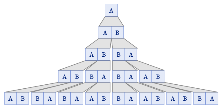
At step n, there are 2ⁿ elements, and the k^th element is determined by whether the number of 1s in the base-2 decomposition of k is even or odd. (This particular case corresponds to the Thue–Morse sequence.)

The evolution of the string substitution system can still be represented by a tree even if the replacements are not the same length. The rules {A  B, B  AB} yield the “Fibonacci tree”:

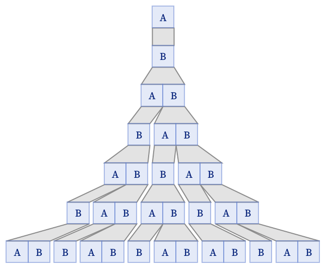
In this case, the number of elements on the t^th step is the t^th Fibonacci number. For any neighbor-independent substitution system, the number of elements on the n^th step is determined by a linear recurrence, and usually, but not always, grows exponentially. (Equivalently, the number of elements of each type on the n^th step can be determined from the n^th power of the transition matrix.)

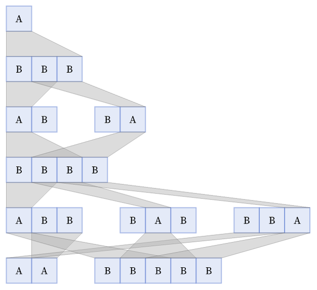
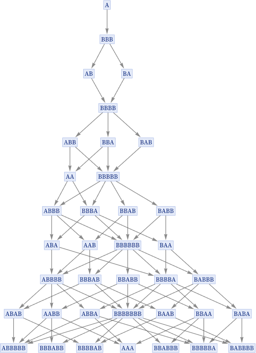
But consider now a substitution system with rules {A  BBB, BB  A}. If one starts with A, the first step is unambiguous: just replace A by BBB. But now there are two possible replacements for BBB: either replace the first BB to get AB, or replace the second one to get BA.

We can represent all the different possibilities as a multiway system [1:5.6] in which there can be multiple outcomes at each step, and there are multiple possible paths of evolution (here shown over the course of 5 steps):

We can represent the possible paths of 5 steps of evolution between states of the system by a graph:

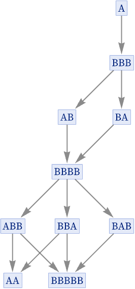
In effect each path through this graph represents a different possible history for the system, based on applying a different sequence of possible updates.

By adding something extra to our model, we can of course force a particular history. For example, we could consider sequential substitution systems (analogous to search-and-replace in a text editor) in which we always do only the first possible replacement in a left-to-right scan of the state reached at each step. With this setup we get the following history for the system shown above:

An alternative strategy (analogous, for example, to the operation of StringReplace in the Wolfram Language) is to scan from left to right, but rather than just doing the first possible replacement at each step, instead keep scanning after the first replacement, and also carry out every subsequent replacement that can independently be done. With this “maximum scan” strategy, the sequence of states reached in the example above becomes:

(The first deviation occurs at BBBB. After replacing the first BB, the maximum scan strategy can continue and replace the second BB as well, thereby in effect “skipping a step” in the multiway evolution graph shown above.)

Note that in both the strategies just described, the evolution obtained can depend on the order in which different replacements are stated in the rule. With the rule {BB  A, A  BBB} instead of {A  BBB, BB  A}, the sequential substitution system updating scheme yields:

instead of:

Given a particular multiway system, one can ask whether it can ever generate a given string. In other words, does there exist any sequence of replacements that leads to a given string? In the case of {A  BBB, BB  A}, starting from A, the strings B and BB cannot be generated, though with this particular rule, all other strings eventually can be generated (it takes 5(k – 1) steps to get all 2^k strings of length k).

One of the applications of multiway systems is as an idealization of derivations in equational logic [1:p777], in which the rules of the multiway system correspond to axioms that define transformations between equivalent expressions in the logical system. Starting from a state corresponding to a particular expression, the states generated by the multiway system are expressions that are ultimately equivalent to the original expression. The paths in the multiway system are then chains of transformations that represent proofs of equivalences between expressions—and the problem of whether a particular equivalence between expression holds is reduced to the (still potentially very difficult) problem of determining whether there is a path in the multiway system that connects the states corresponding to these expressions.

Thus, for example, with the transformations {A  BBB, BB  A}, it is possible to see that A can be transformed to AAA, but the path required is 10 steps long:

In general, there is no upper bound on how long a path may be required to reach a particular string in a multiway system, and the question of whether a given string can ever be reached is in general undecidable [52][53][1:p778].