5.2 The Phenomenon of Causal Invariance

Consider the rule {BA  AB}, starting from BABABA:

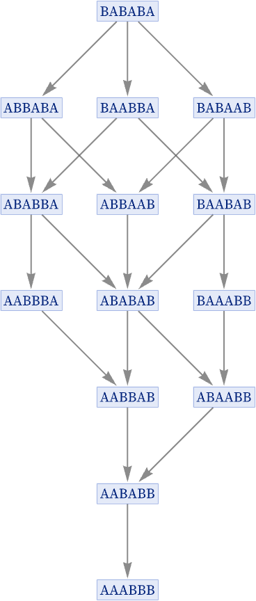
As before, there are different possible paths through this graph, corresponding to different possible histories for the system. But now all these paths converge to a single final state. And in this particular case, there is a simple interpretation: the rule is effectively sorting As in front of Bs by repeatedly doing the transposition BA  AB. And while there are multiple different possible sequences of transpositions that can be used, all of them eventually lead to the same answer: the sorted state AAABBB.

There are many practical examples of systems that behave in this kind of way, allowing operations to be carried out in different orders, generating different intermediate states, while always leading to the same final answer. Evaluation or simplification of (parenthesized) arithmetic (e.g. [54]), algebraic or Boolean expressions are examples, as is lambda function evaluation [55].

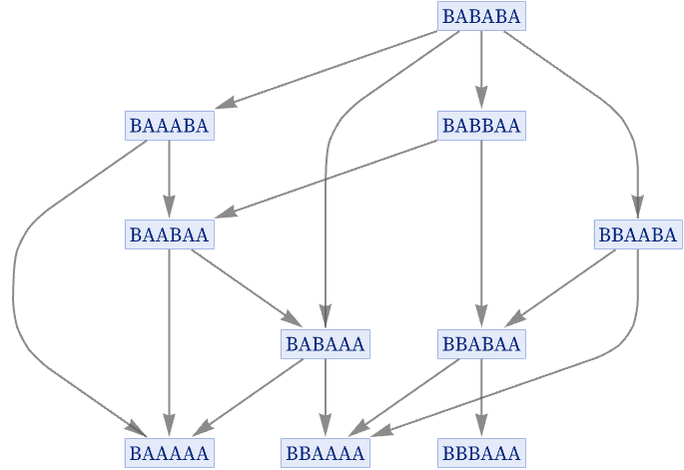
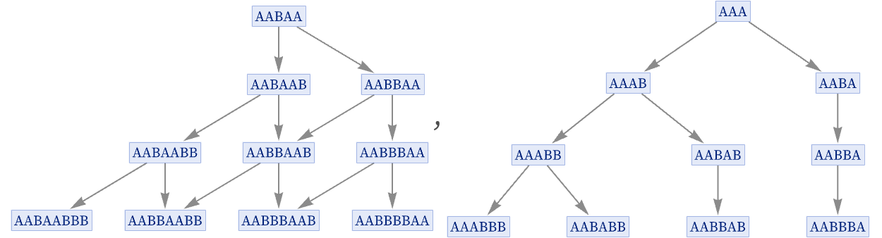
Many substitution systems, however, do not have this property. For example, consider the rule {AB  AA, AB  BA}, again starting from BABABA. Like the sorting rule, after a limited number of steps this rule gets into a final state that no longer changes. But unlike the sorting rule, it does not have a unique final state. Depending on what path is taken, it goes in this case to one of three possible final states:

But what about systems that do not “terminate” at particular final states? Is there some way to define a notion of “path independence” [55]—or what we will call “causal invariance” [1:9.10]—for these?

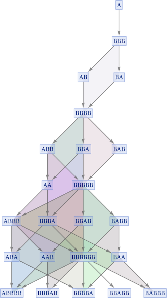
Consider again the rule {A  BBB, BB  A} that we discussed above:

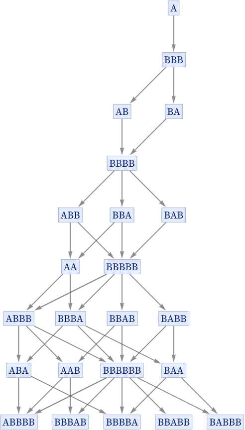
The state BBB at step 2 has two possible successors: AB and BA. But after another step, AB and BA converge again to the state BBBB. And in fact the same kind of thing happens throughout the graph: every time two paths diverge, they always reconverge after just one more step. This means that the graph in effect consists of a collection of “diamonds” of edges [56]:

There is no need, however, for reconvergence to happen in just one step. Consider for example the rule {A  AA, AA  AB}:

As the picture indicates, there are paths from AAA leading to both ABA and AAB—but these only reconverge again (to ABAB) after two more steps. (In general, it can take an arbitrary number of steps for reconvergence to occur.)

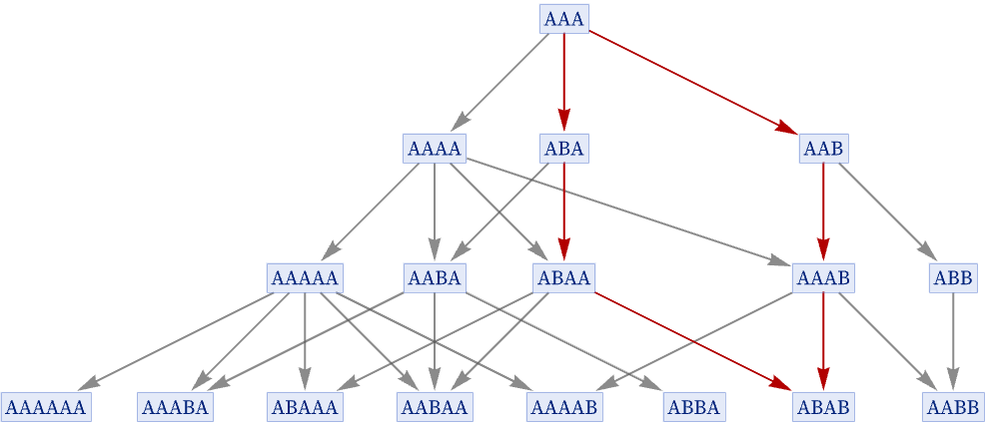
Whether a system is causal invariant may depend on its initial conditions. Consider, for example, the rule AA  AAB. With initial condition AABAA the rule is causal invariant, but with initial condition AAA it is not:

When a system is causal invariant for all possible initial conditions, we will say that it is totally causally invariant. (This is essentially the confluence property discussed in the theory of term-rewriting systems.) Later, we will discuss how to systematically test for causal invariance—and we will see that it is often easier to test for total causal invariance than for causal invariance for specific initial conditions.

Causal invariance may at first seem like a rather obscure property. But in the context of our models, we will see in what follows that it may in fact be the key to a remarkable range of fundamental features of physics, including relativistic invariance, general covariance, and local gauge invariance, as well as the possibility of objective reality in quantum mechanics.