5.18 The Relationship between Graphs, and the Multiway Causal Graph

In the course of this section, we have seen various ways of describing and relating the possible behaviors of systems. In many ways the most general is the combined multiway evolution and multiway causal graph.

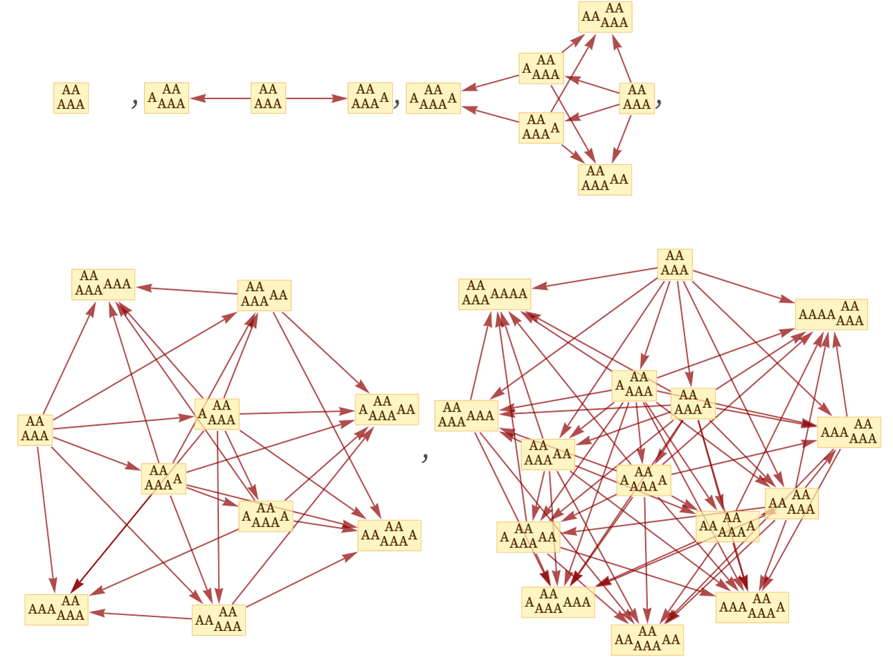
For the rule

starting from AA this graph has the form:

Continuing for another step, we have:

There are several different kinds of descriptions that we can derive from this graph. The standard multiway graph gives the evolution relationship between states:

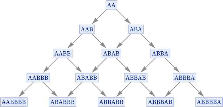
Each possible path through this graph corresponds to a possible evolution history for the system.

The multiway causal graph gives the causal relationships between all events that can happen on any branch. The full multiway causal graph for the rule shown here is infinite. But truncating to show only the part contained in the graph above, one gets:

Continuing for more steps one gets:

From the multiway causal graph, one can project out the specific causal graph for each possible evolution history, corresponding to each possible branch in the multiway system. But for rules like the one shown here that have the property of causal invariance, every one of these specific causal graphs (at least if extended far enough) must have exactly the same structure. For the particular rule shown here, this structure is extremely simple:

(In effect, the nodes here are “generic events” in the system, and could be labeled just by copies of the underlying local rule.)

The multiway graph and multiway causal graph effectively give two different “vertical views” of the original graph—using respectively states as nodes and events as nodes. But an alternative is to view the graph in terms of “horizontal slices”. To get such slices we have to do foliations.

But now if we look at horizontal slices associated with states, we get the branchial graphs, which for this rule with this initial condition are rather trivial:

In principle we could also ask about horizontal slices associated with events. But by construction the events analog of the branchial graph must just consist of a collection of complete graphs.

However, a particular sequence of slices through any particular causal graph defines an actual sequence of states for the underlying system, and thus a possible evolution history, such as:

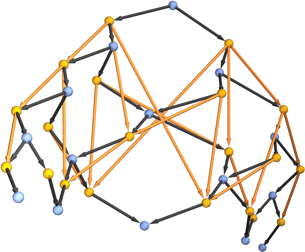
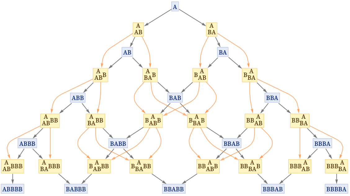
As a slightly cleaner example with similar behavior, consider the rule:

The combined multiway evolution and multiway causal graph in this case is

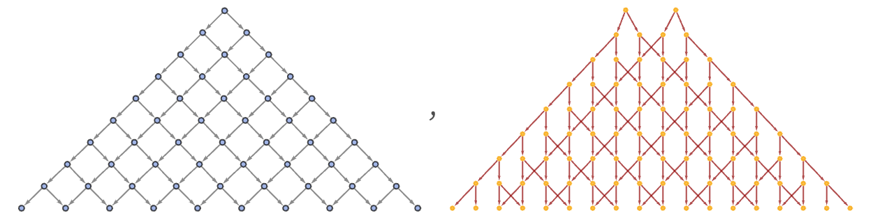
and the individual multiway evolution and causal graphs are both regular 2D grids:

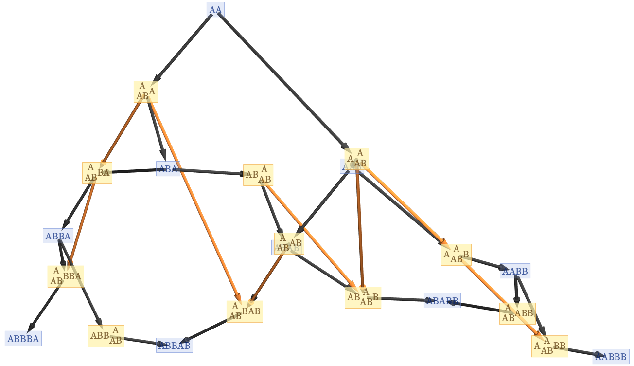
The rules we have used as an example so far have behavior that is in a sense fairly trivial. But consider now the related rule with slightly less trivial behavior:

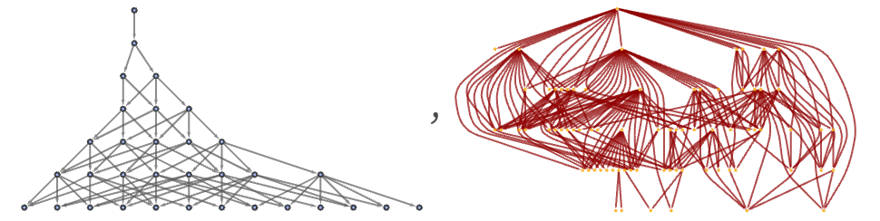
For this rule, the combined multiway evolution and causal graph has the form:

On their own, the state evolution graph and the event causal graph have the forms:

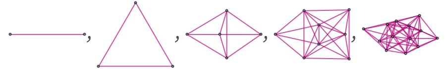
The sequence of branchial graphs is:

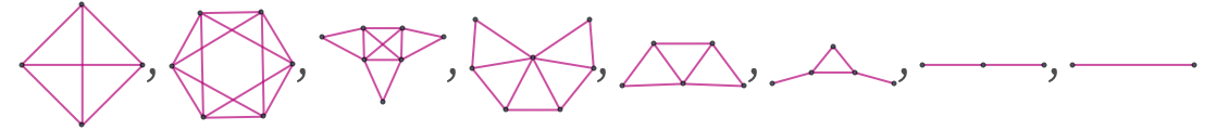
This rule is causal invariant, and so the multiway causal graph decomposes into many identical copies of causal graphs for all individual possible paths of evolution. In this case, these graphs all have the form:

But even though the multiway causal graph can be decomposed into identical pieces, it still contains more information than any of them. Because in effect it describes not only “spatial” causal relationships between events happening in different places in the underlying string, but also “branchial” causal relationships between events happening on different branches of the multiway system.

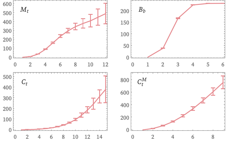
And just like for other graphs, we can study the large-scale structure of multiway causal graphs. We can define a quantity which is the multiway analog of the cone volume C_t for individual causal graphs. For the rule shown here, the various graph growth rates (as computed with our standard foliation) have the forms:

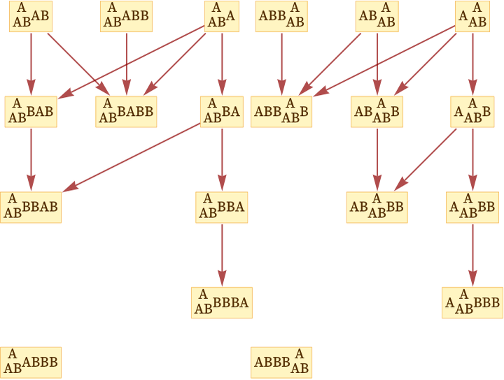
As another example, consider the “sorting” rule

starting from BABABABA. The combined multiway evolution and causal graph has the (terminating) form:

The multiway evolution and causal graphs on their own are:

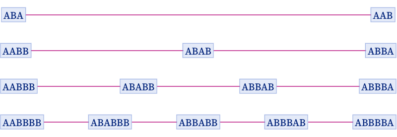
The branchial graphs are

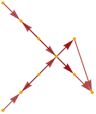
and the causal graph for a single (finite) path of evolution is:

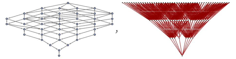
Earlier in this section we looked at the multiway evolution graphs generated by all 12 inequivalent 2: 12, 11 rules. The pictures below now compare these with the multiway causal graphs for the same rules (starting from all possible length-3 strings of As and Bs, and run for 4 steps of our standard multiway foliation):

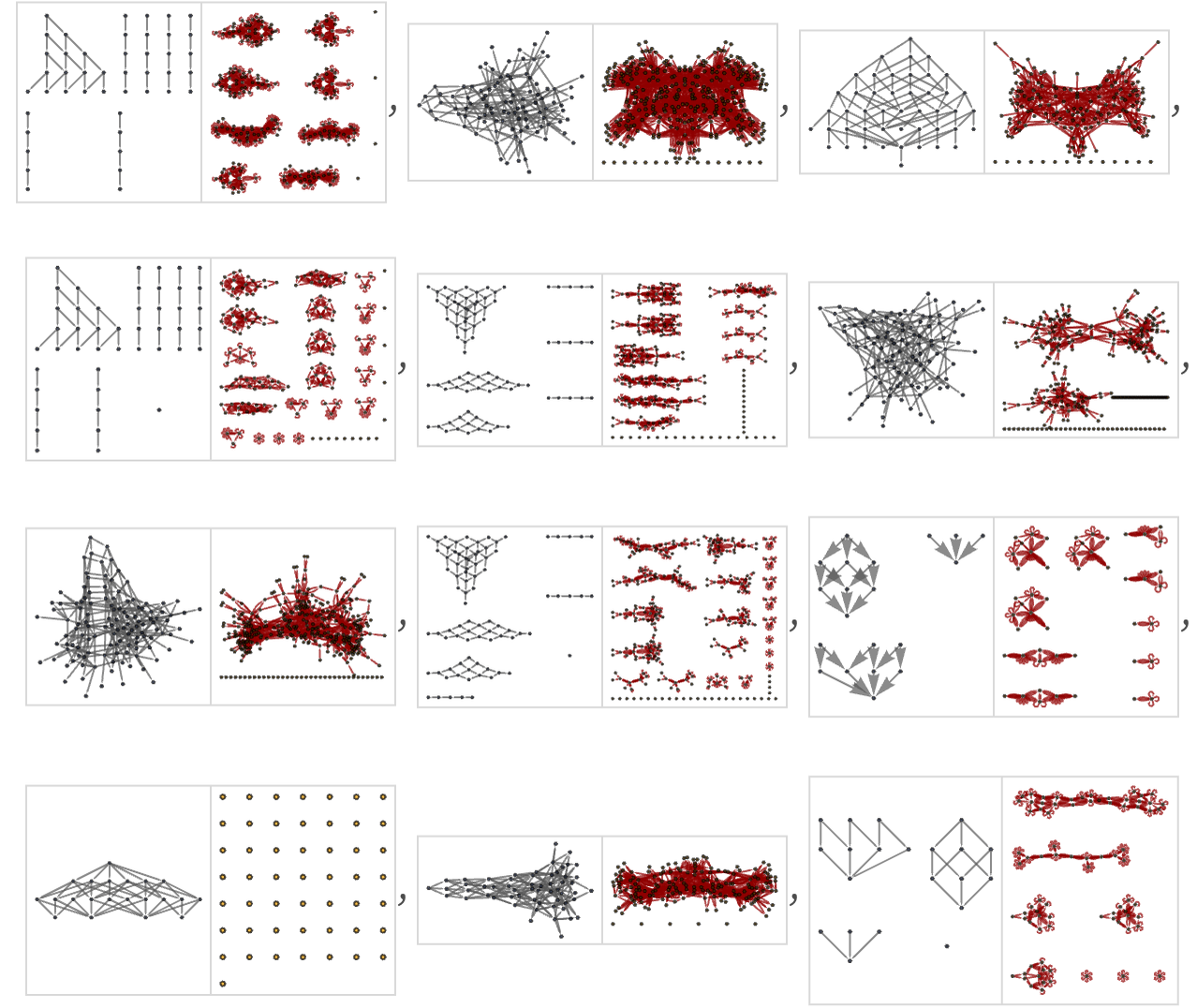
The multiway causal graph is in some ways a kind of dual to the multiway evolution graph—resulting in many similarities among the graphs in the pictures above. Like M_t for multiway evolution graphs, for multiway causal graphs typically seems to grow either polynomially or exponentially.

But even in a case like the rule

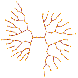
where the causal graph for a single evolution has the fairly regular form

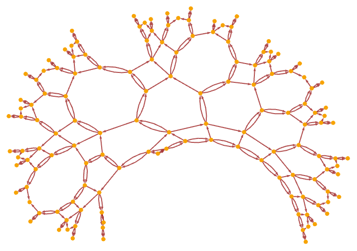
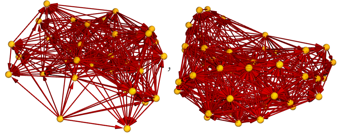
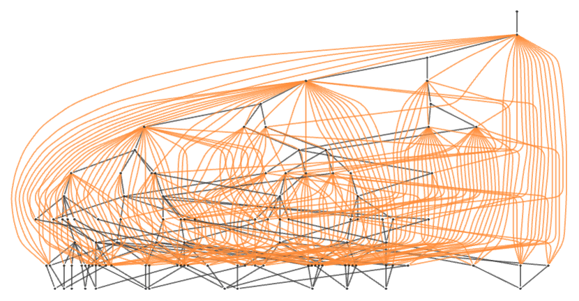
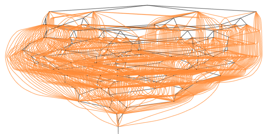
the full multiway causal graph is quite complex. This shows how it builds up over the first few steps (in our standard multiway foliation):

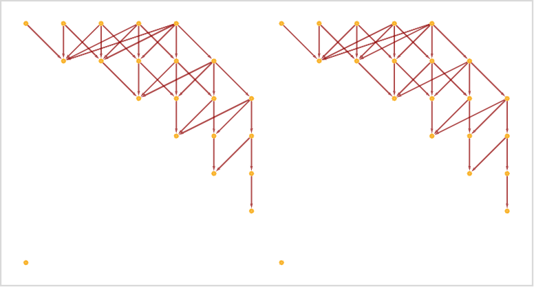
And here are 3D renderings after 8 and 9 steps: