5.19 Weighted Multiway Graphs

In a multiway system, there are in general multiple paths that can produce the same state. But in our usual construction of the multiway graph, we record only what states are produced, not how many paths can do it.

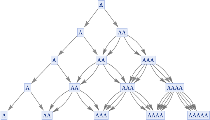
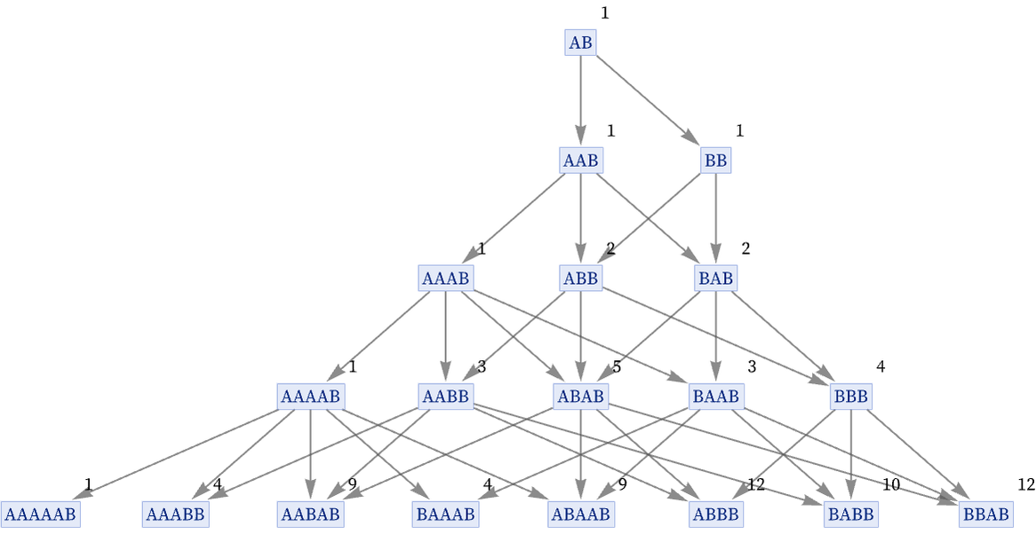
Consider the rule:

The full form of its multiway graph—including an edge for every possible event—is:

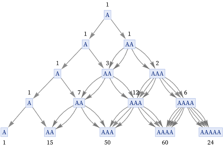
Here is the same graph, with a count included at each node for the number of distinct paths from the root that reach it:

An alternative weighting scheme might be to start with weight 1 for the initial state, then at each state we reach, to distribute the weight to its successors, dividing it equally among possible events:

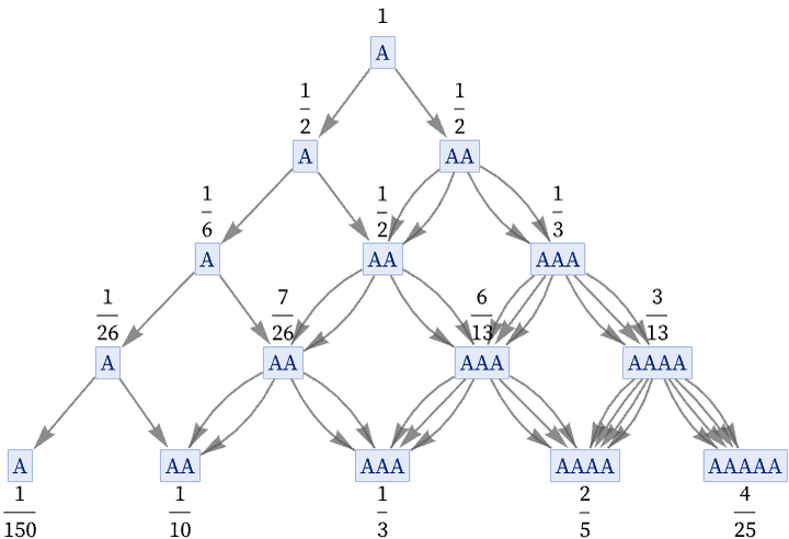
This approach has the feature that it gives normalized weights (summing to 1) at each successive layer in a graph like this. But in general the approach is not robust, and if we even took a different foliation through the graph above, the weights on each slice would no longer be normalized. In addition, if we were to combine identical states from different steps, we would not know what weights to assign. Pure counting of paths, however, still works even in this case, although any normalization has to be done only after all the counts are known:

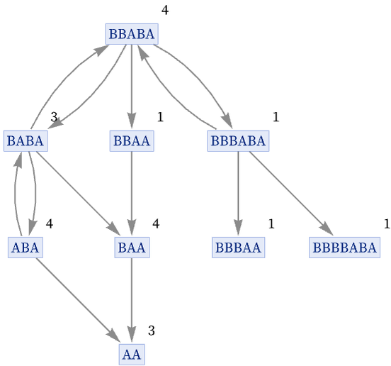
Note that even the counting of paths becomes difficult to define if there is a loop in the multiway graph—though one can adopt the convention that one counts paths only to the first encounter with any given state:

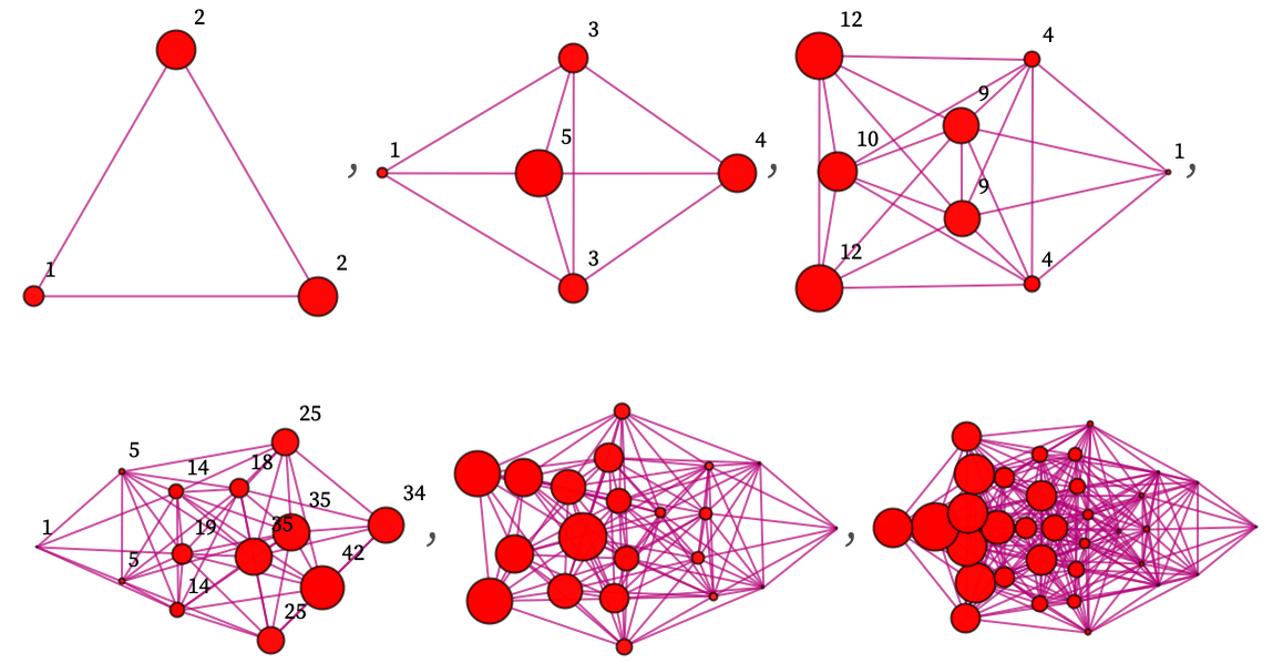
Weights on the multiway graph can also be inherited by branchial graphs. Consider for example the rule:

The multiway graph for this rule, weighted with path counts, is:

The corresponding weighted branchial graphs are:

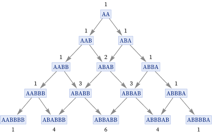
The weights in effect define a measure on the branchial graph. A case with a particular straightforward limiting measure is the rule:

With initial condition A this gives weights that reproduce Pascal’s triangle, and yield a limiting Gaussian:

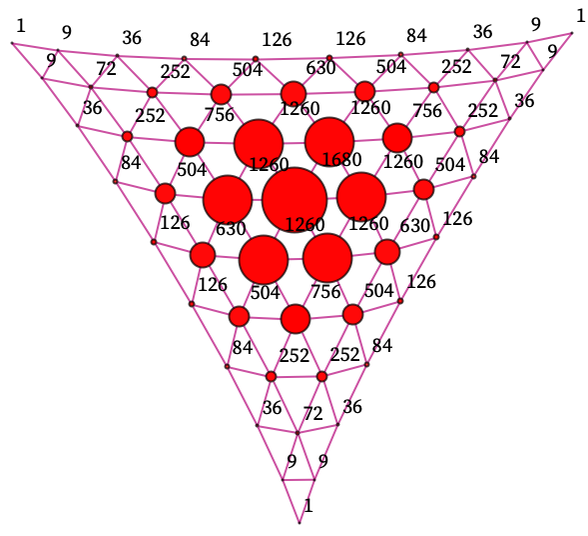
With initial condition AAA, the weights in the branchial graph limit to a 2D Gaussian:

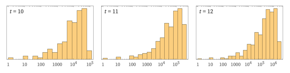
In general, after sufficiently many steps one can expect that the weights will define an invariant measure, although a complexity is that the branchial graph will typically continue to grow. As one indication of the limiting measure, one can compute the distribution of values of the weights.

The results for the rule {A  B, B  AB} above illustrate slow convergence to a limiting form:

We discussed in a previous subsection probing the structure of the branchial graph by computing the number of nodes B_b at most graph distance b from a given point. We can now generalize this to computing a path-weighted quantity (cf. [1:p959]). At least for simple multiway graphs, this may be related in the limit to the results of solving a PDE on the multiway graph.