A Class of Models with the Potential to Represent Fundamental Physics
  1. Introduction
  2. Basic Form of Models
  3. Typical Behaviors
  4. Limiting Behavior and Emergent Geometry
  5. The Updating Process for String Substitution Systems
  6. The Updating Process in Our Models
  7. Equivalence and Computation in Our Models
  8. Potential Relation to Physics
  9. Additional Material
  10. References
  11. Index

5.12 Typical Causal Graphs

Any causal invariant system always ultimately has a unique causal graph. The graph can be found by analyzing any possible evolution for the system, with any updating schemethough for visualization purposes, it is usually useful to use an updating scheme where as much happens as possible at each step.

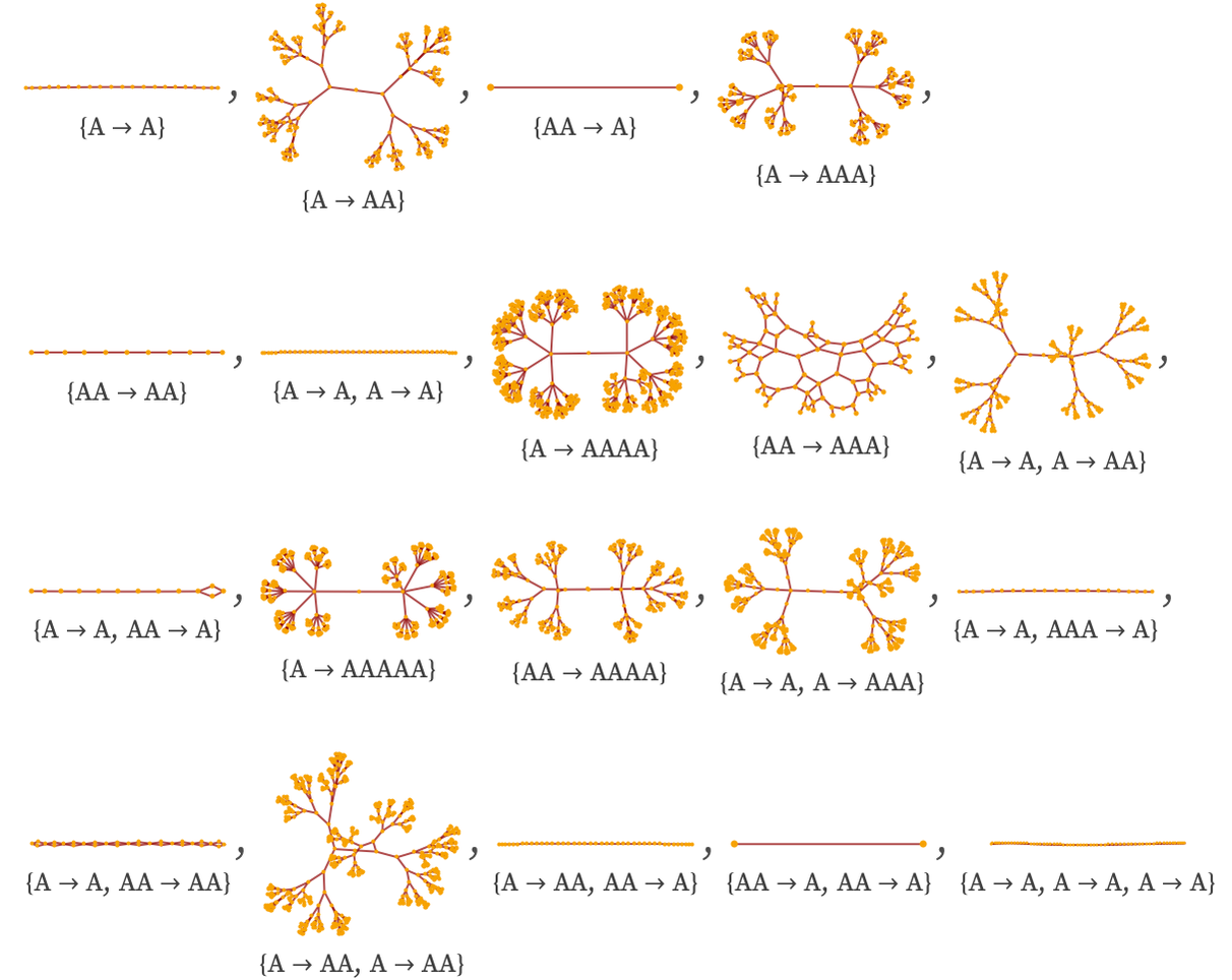
The trivial causal invariant rule A A starting from A has causal graph:

ResourceFunction["SubstitutionSystemCausalGraph"]["A" -> "A", "A", 5]

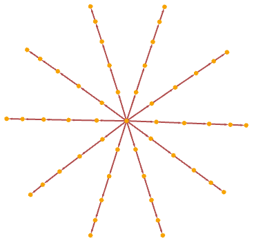
Starting from a string of 10 As it has causal graph:

ResourceFunction["SubstitutionSystemCausalGraph", ResourceVersion -> "3.0.0"]["A" -> "A", StringRepeat["A", 10], 5, "IncludeInitializationEvents" -> True]

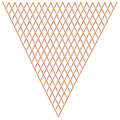
A AA has a causal graph starting from A that is a binary tree

TreePlot[ResourceFunction["SubstitutionSystemCausalGraph"][ "A" -> "AA", "A", 6]]

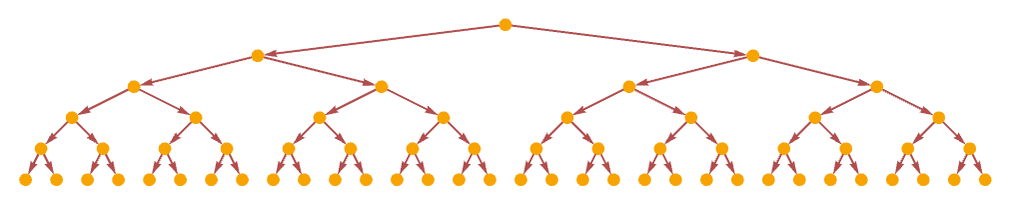
which can also be rendered:
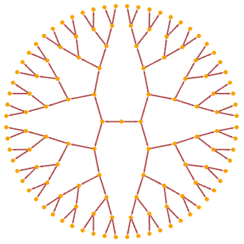
TreePlot[ResourceFunction["SubstitutionSystemCausalGraph"][ "A" -> "AA", "A", 7], Center]

The rule

{"A" -> "A", "A" -> "AA"}

starting from A gives a “two-step binary tree” with  nodes at level t:

TreePlot[ResourceFunction[ "SubstitutionSystemCausalGraph"][{"A" -> "A", "A" -> "AA"}, "A", 7], Center]

One does not have to go beyond rules involving just a single element (all of which are causal invariant) to find a range of causal graph structures. For example, here are all the forms obtained by rules allowing up to 6 instances of a single element A, with initial condition AA:

bigcg[rule_, init_, maxt_, maxv_] := Catch[(Do[ With[{w = ResourceFunction["SubstitutionSystemCausalGraph"][rule, init, t, "IncludeInitializationEvents" -> True]}, If[VertexCount[w] > maxv, Throw[w], w]], {t, maxt}]; ResourceFunction["SubstitutionSystemCausalGraph"][rule, init, maxt, "IncludeInitializationEvents" -> True])]; Labeled[UndirectedGraph[bigcg[#, "AA", 10, 200], GraphLayout -> "SpringElectricalEmbedding", ImageSize -> Tiny], Style[#, GrayLevel[.25], FontSize -> .85 Inherited, FontFamily -> "Source Serif Pro"]] & /@ {{"A" -> "A"}, {"A" -> "AA"}, {"AA" -> "A"}, {"A" -> "AAA"}, {"AA" -> "AA"}, {"A" -> "A", "A" -> "A"}, {"A" -> "AAAA"}, {"AA" -> "AAA"}, {"A" -> "A", "A" -> "AA"}, {"A" -> "A", "AA" -> "A"}, {"A" -> "AAAAA"}, {"AA" -> "AAAA"}, {"A" -> "A", "A" -> "AAA"}, {"A" -> "A", "AAA" -> "A"}, {"A" -> "A", "AA" -> "AA"}, {"A" -> "AA", "A" -> "AA"}, {"A" -> "AA", "AA" -> "A"}, {"AA" -> "A", "AA" -> "A"}, {"A" -> "A", "A" -> "A", "A" -> "A"}}

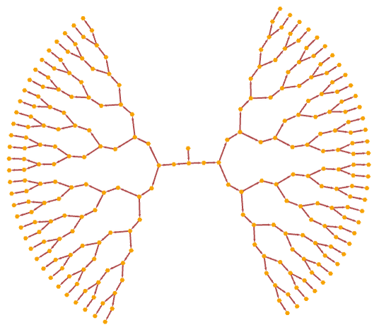
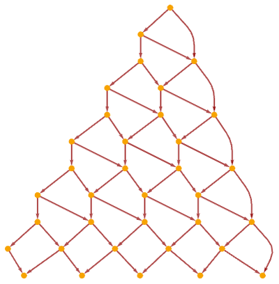
A notable case is the rule:

{"AA" -> "AAA"}

Shown in layered form, the first few steps give:

Table[Show[ LayeredGraphPlot[ ResourceFunction["SubstitutionSystemCausalGraph"]["AA" -> "AAA", "AA", t, "IncludeInitializationEvents" -> True], ImageSize -> {Automatic, 100}]] /. Arrowheads[Medium] -> Arrowheads[0.01], {t, 8}]

After a few more steps, this can be rendered as:

ResourceFunction["SubstitutionSystemCausalGraph"][ "AA" -> "AAA", "AA", 14, "IncludeInitializationEvents" -> True]

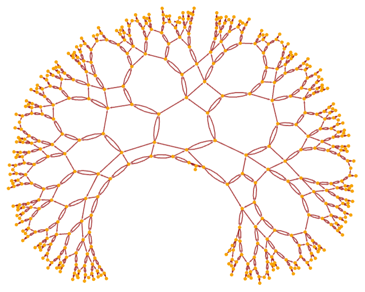
Running the underlying substitution system AA AAA updating as much as possible at each step (the StringReplace scheme), one gets strings with successive lengths

which follow the recurrence:

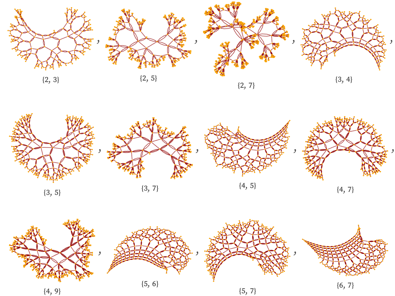
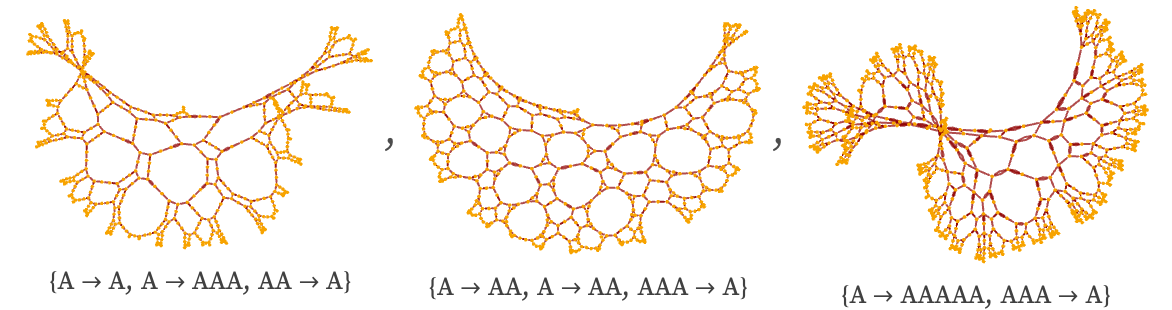
Other rules of the form Ap Aq for non-commensurate p and q give similar results, analogous to tessellations in hyperbolic space:

bigcg[rule_, init_, maxt_, maxv_] := Catch[(Do[ With[{w = ResourceFunction["SubstitutionSystemCausalGraph"][rule, init, t, "IncludeInitializationEvents" -> True]}, If[VertexCount[w] > maxv, Throw[w], w]], {t, maxt}]; ResourceFunction["SubstitutionSystemCausalGraph"][rule, init, maxt, "IncludeInitializationEvents" -> True])]; Labeled[Graph[ bigcg[StringRepeat["A", #1] -> StringRepeat["A", #2], StringRepeat["A", #1], 50, 200], ImageSize -> 80, ResourceFunction["WolframPhysicsProjectStyleData"][ "CausalGraph"]], Style[{#1, #2}, GrayLevel[.25], FontSize -> .85 Inherited, FontFamily -> "Source Serif Pro"], ImageSize -> 150] & @@@ {{2, 3}, {2, 5}, {2, 7}, {3, 4}, {3, 5}, {3, 7}, {4, 5}, {4, 7}, {4, 9}, {5, 6}, {5, 7}, {6, 7}}

Rules that involve multiple replacements can give similar behavior even starting from a single A:

bigcg[rule_, init_, maxt_, maxv_] := Catch[(Do[ With[{w = ResourceFunction["SubstitutionSystemCausalGraph"][rule, init, t, "IncludeInitializationEvents" -> True]}, If[VertexCount[w] > maxv, Throw[w], w]], {t, maxt}]; ResourceFunction["SubstitutionSystemCausalGraph"][rule, init, maxt, "IncludeInitializationEvents" -> True])]; Labeled[Graph[bigcg[#1, "A", 100, 500], ImageSize -> 200, ResourceFunction["WolframPhysicsProjectStyleData"][ "CausalGraph"]], Style[#1, GrayLevel[0.25], FontSize -> .85 Inherited, FontFamily -> "Source Serif Pro"]] & /@ {{"A" -> "A", "A" -> "AAA", "AA" -> "A"}, {"A" -> "AA", "A" -> "AA", "AAA" -> "A"}, {"A" -> "AAAAA", "AAA" -> "A"}}

Rules just containing only As cannot progressively grow to produce ordinary tilings. One can get these with the “sorting rule”

{"BA" -> "AB"}

which when started with 20 BAs yields:

VertexDelete[ ResourceFunction["SubstitutionSystemCausalGraph"]["BA" -> "AB", StringRepeat["BA", 20], 20, "IncludeInitializationEvents" -> True], 1] // LayeredGraphPlot

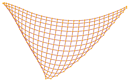
There are also rules which “grow” grid-like tilings. For example, the rule

{"A" -> "AB", "BB" -> "BB"}

starting from a single A produces

LayeredGraphPlot[ ResourceFunction["SubstitutionSystemCausalGraph"][{"A" -> "AB", "BB" -> "BB"}, "A", 10], AspectRatio -> 1]

which is equivalent to a square grid:

ResourceFunction["SubstitutionSystemCausalGraph"][{"A" -> "AB", "BB" -> "BB"}, "A", 30]

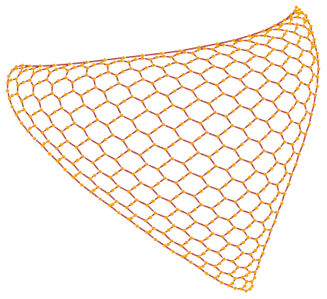
There is also a simple rule that generates essentially a hexagonal grid:

{"A" -> "B", "B" -> "AB", "BA" -> "A"}
ResourceFunction["SubstitutionSystemCausalGraph"][{"A" -> "B", "B" -> "AB", "BA" -> "A"}, "A", 20]

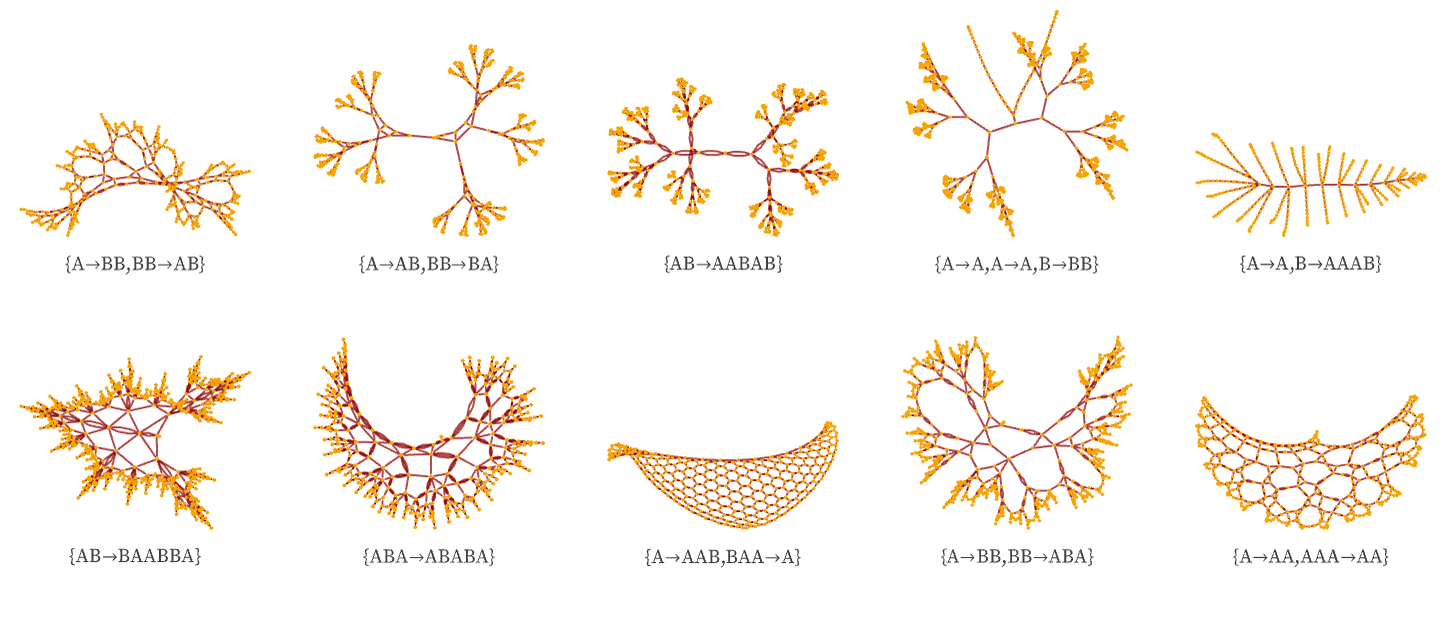
Other forms of causal graphs produced by simple causal invariant substitution systems include (starting from A, AB or ABA):

bigcg[rule_, init_, maxt_, maxv_] := Catch[(Do[ With[{w = ResourceFunction["SubstitutionSystemCausalGraph"][rule, init, t, "IncludeInitializationEvents" -> True]}, If[VertexCount[w] > maxv, Throw[w], w]], {t, maxt}]; ResourceFunction["SubstitutionSystemCausalGraph"][rule, init, maxt, "IncludeInitializationEvents" -> True])] GraphicsGrid[ Partition[ Labeled[bigcg[#1, #2, 50, 300], Text[Style[#1, GrayLevel[.25], FontSize -> .95 Inherited, FontFamily -> "Source Serif Pro"]], ImageSize -> 120] & @@@ {{{"A" -> "BB", "BB" -> "AB"}, "A"}, {{"A" -> "AB", "BB" -> "BA"}, "A"}, {{"AB" -> "AABAB"}, "AB"}, {{"A" -> "A", "A" -> "A", "B" -> "BB"}, "ABA"}, {{"A" -> "A", "B" -> "AAAB"}, "ABA"}, {{"AB" -> "BAABBA"}, "AB"}, {{"ABA" -> "ABABA"}, "ABA"}, {{"A" -> "AAB", "BAA" -> "A"}, "A"}, {{"A" -> "BB", "BB" -> "ABA"}, "A"}, {{"A" -> "AA", "AAA" -> "AA"}, "A"}}, 5], Alignment -> Bottom, ImageSize -> Full]

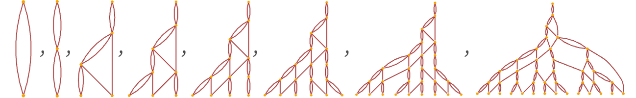
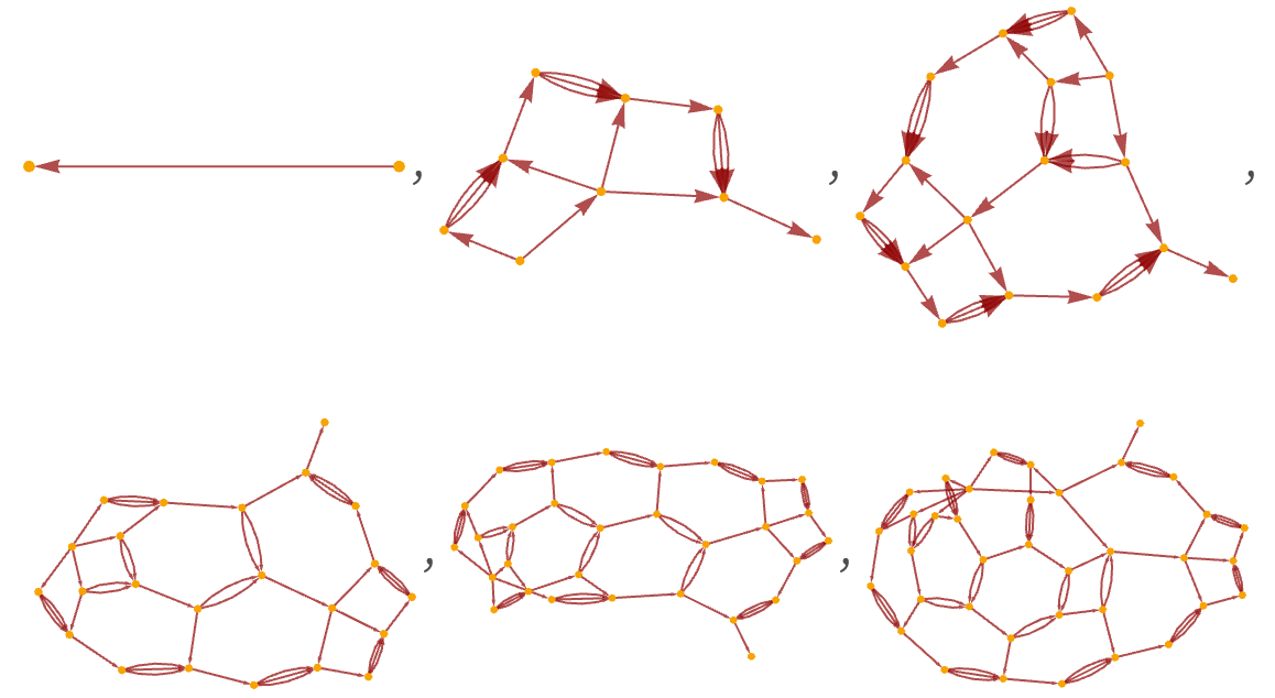
When rules terminate they yield finite causal graphs. But these can often be quite complicated. For example, the rule

{"A" -> "BBB", "BBBB" -> "A"}

started from strings consisting of from 1 to 6 As yields the following finite causal graphs:

Table[Graph[ ResourceFunction["SubstitutionSystemCausalGraph"][{"A" -> "BBB", "BBBB" -> "A"}, StringRepeat["A", n], 50, "IncludeInitializationEvents" -> True], GraphLayout -> "SpringElectricalEmbedding"], {n, 6}]

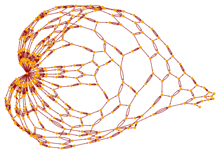
With a string of 50 As, the rule gives the finite causal graph:

ResourceFunction["SubstitutionSystemCausalGraph"][{"A" -> "BBB", "BBBB" -> "A"}, StringRepeat["A", 50], 1000, "IncludeInitializationEvents" -> True]

Compared to the hypergraphs we studied in previous sections, or even the multiway graphs from earlier in this section, the causal graphs here may seem to have rather simple structures. But there is a good reason for this. While there can be many updating events in the evolution of a string substitution system, all of them are in a sense arranged on the same one-dimensional structure that is the underlying string. And since the updating rules we consider involve strings of limited length, there is inevitably a linear ordering to the events along the string. This greatly simplifies the possible forms of causal graphs that can occur, for example requiring them always to remain planar. In the next section, we will see that for our hypergraph-based modelswhich have no simplifying underlying structurecausal graphs can be considerably more complex.