A Class of Models with the Potential to Represent Fundamental Physics
  1. Introduction
  2. Basic Form of Models
  3. Typical Behaviors
  4. Limiting Behavior and Emergent Geometry
  5. The Updating Process for String Substitution Systems
  6. The Updating Process in Our Models
  7. Equivalence and Computation in Our Models
  8. Potential Relation to Physics
  9. Additional Material
  10. References
  11. Index

5.13 Limits of Causal Graphs

Much as we did for hypergraphs in section 4, we can consider the limiting structures of causal graphs after a large number of steps. And much as for hypergraphs, we can potentially describe these limiting structures in terms of emergent geometry. But one difference from what we did for hypergraphs is that for causal graphs, it is essential to take account of the directedness of their edges. It is still perfectly possible to have a limit that is like a manifold, but now to measure its properties we must generate the analog of cones, rather than balls.

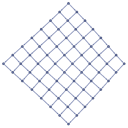
Consider for example the simple directed grid graph:

LayeredGraphPlot[ ResourceFunction["GeneralizedGridGraph"][{8 -> "Directed", 8 -> "Directed"}], VertexStyle -> ResourceFunction["WolframPhysicsProjectStyleData"]["SpatialGraph", "VertexStyle"], EdgeStyle -> ResourceFunction["WolframPhysicsProjectStyleData"]["SpatialGraph", "EdgeLineStyle"], AspectRatio -> 1]

Now consider starting from a particular node, and constructing progressively larger “cones”:

Table[With[{g = ResourceFunction["GeneralizedGridGraph"][{8 -> "Directed", 8 -> "Directed"}]}, LayeredGraphPlot[ HighlightGraph[g, Subgraph[g, VertexOutComponent[g, 10, t]], GraphHighlightStyle -> "Thick", ImageSize -> Tiny], VertexStyle -> ResourceFunction["WolframPhysicsProjectStyleData"]["SpatialGraph", "VertexStyle"], EdgeStyle -> ResourceFunction["WolframPhysicsProjectStyleData"]["SpatialGraph", "EdgeLineStyle"], AspectRatio -> 1]], {t, 1, 5}]

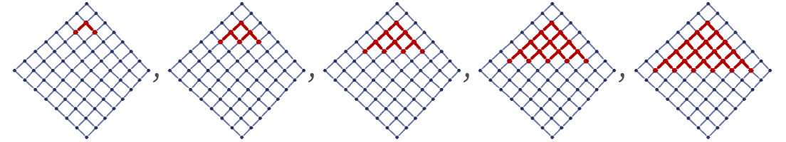
We can call the number of nodes in this cone after t steps Ct. In this case the result (for t below the diameter of the graph) is:

And in the limit of large graphs, we will have:

We can also set up a 3D directed grid graph

Graph3D[ResourceFunction["GeneralizedGridGraph"][{5 -> "Directed", 5 -> "Directed", 5 -> "Directed"}], VertexStyle -> ResourceFunction["WolframPhysicsProjectStyleData"]["SpatialGraph3D", "VertexStyle"], EdgeStyle -> ResourceFunction["WolframPhysicsProjectStyleData"]["SpatialGraph3D", "EdgeLineStyle"]]

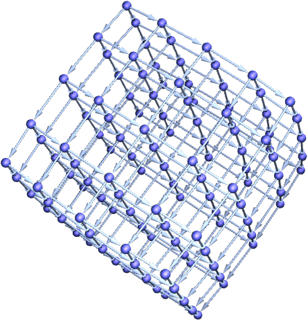
and generate a similar cone

Table[With[{g = Graph3D[ResourceFunction["GeneralizedGridGraph"][{5 -> "Directed", 5 -> "Directed", 5 -> "Directed"}], BaseStyle -> {Graphics3DBoxOptions -> {Method -> {"ShrinkWrap" -> True}}}, VertexStyle -> ResourceFunction["WolframPhysicsProjectStyleData"][ "SpatialGraph3D", "VertexStyle"], EdgeStyle -> ResourceFunction["WolframPhysicsProjectStyleData"][ "SpatialGraph3D", "EdgeLineStyle"]]}, GraphPlot3D[ HighlightGraph[g, Subgraph[g, VertexOutComponent[g, 1, t]], GraphHighlightStyle -> "Thick"], ViewPoint -> {-1.4301580899899289`, -0.1054485183561964`, 3.064886367814122`}, ImageSize -> Tiny]], {t, 1, 5}]

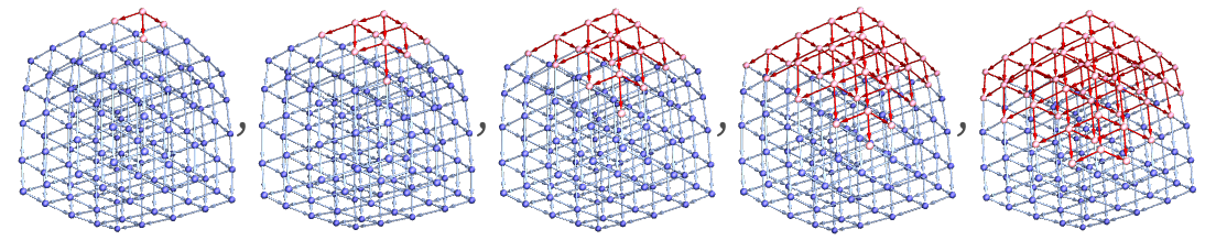
for which now Ct~ t3.

In general, we can think about the limits of these grid graphs as generating a d-dimensional “directed space”. There is also nothing to prevent having cyclic versions, such as

Graph3D[ResourceFunction[ "GeneralizedGridGraph"][{10 -> {"Directed", "Circular"}, 6 -> {"Directed", "Circular"}}], VertexStyle -> ResourceFunction["WolframPhysicsProjectStyleData"]["SpatialGraph3D", "VertexStyle"], EdgeStyle -> ResourceFunction["WolframPhysicsProjectStyleData"]["SpatialGraph3D", "EdgeLineStyle"]]

and in general a family of graphs that are going to behave like d-dimensional directed space in the limit will have Ct~ td.

In direct analogy to what we did with hypergraphs in section 4, we can compute Ct for causal graphs, and then estimate effective dimension by looking at its growth rate. (There are some additional subtleties, though, because whereas at any given step in the evolution of the system, Vr can be computed for any r for any point in a hypergraph, Ct can be computed only until t “reaches the edge of the causal graph” from that starting pointand later we will see that the cutoff can also depend on the foliation one uses.)

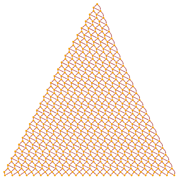
Consider the substitution system:

{"A" -> "AB", "BB" -> "BB"}

This generates the causal graph:

LayeredGraphPlot[ ResourceFunction["SubstitutionSystemCausalGraph"][{"A" -> "AB", "BB" -> "BB"}, "A", 50], AspectRatio -> 1]

The log differences of Ct averaged over all points for causal graphs obtained from 10 through 100 steps of evolution have the form (the larger error bars for larger t in each case are the result of fewer starting points being able to contribute):

ListLinePlot[ Table[ResourceFunction["LogDifferences"]@ ResourceFunction["RaggedMeanAround"][ Values[ResourceFunction["GraphNeighborhoodVolumes"][ ResourceFunction["SubstitutionSystemCausalGraph"][{"A" -> "AB", "BB" -> "BB"}, "A", t]]]], {t, 10, 100, 10}], Frame -> True, PlotRange -> {0, Automatic}, PlotStyle -> ResourceFunction["WolframPhysicsProjectStyleData"][ "GenericLinePlot", "PlotStyles"]]

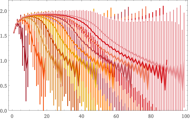
As expected, for t small compared to the number of steps, the limiting estimated dimension is 2.

Most of the other causal graphs shown in the previous subsection do not have finite dimension, however. For example, for the rule AA AAA the causal graph has the form
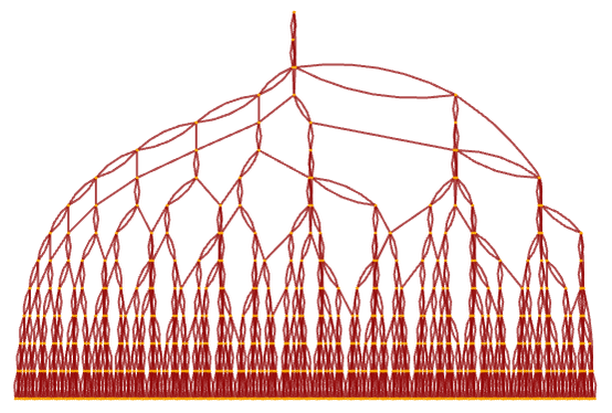
LayeredGraphPlot[ ResourceFunction["SubstitutionSystemCausalGraph"][{"AA" -> "AAA"}, "AA", 15], AspectRatio -> 2/3]

which increases exponentially, with  .

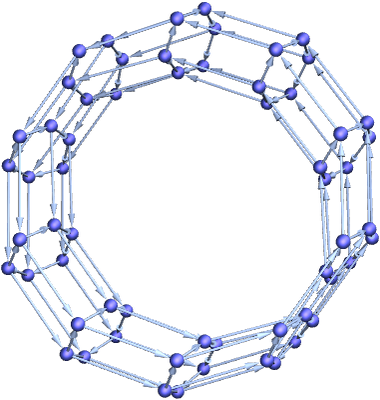
The limits of the grid graphs we showed above essentially correspond to flat d-dimensional directed space. But we can also consider d-dimensional directed space with curvature. Although we cannot construct a complete sphere graph that is consistently directed, we can construct a partial sphere graph:

curvedDirectedGraph[n_, neighborhoodSize_, v_ : 1] := With[{graph = NeighborhoodGraph[ResourceFunction["BuckyballGraph"][n], v, neighborhoodSize]}, With[{center = GraphCenter[graph][[1]]}, {HighlightGraph[ Graph3D[Select[ Reap[BreadthFirstScan[graph, center, {"VisitedVertex" -> (Sow[#1 -> #2] &)}]][[2, 1]], #[[1]] != #[[2]] &], DirectedEdges -> True], center], center, ResourceFunction["GraphNeighborhoodVolumes"][ graph, {center}][[1]]}]]; GraphPlot3D[ First[curvedDirectedGraph[7, 25]], {ViewPoint -> {1.9859617640476468`, -1.698082088118901`, \ -2.149993742723572`}, ViewCenter -> {{0.5`, 0.5`, 0.5`}, {0.5020373719047886`, 0.427847916967363`}}, ViewVertical -> {0.4825436620397217`, -0.6396841189361542`, 0.598294110121578`}, ViewAngle -> 0.12626201637818915`}, VertexStyle -> ResourceFunction["WolframPhysicsProjectStyleData"]["SpatialGraph3D", "VertexStyle"], EdgeStyle -> ResourceFunction["WolframPhysicsProjectStyleData"]["SpatialGraph3D", "EdgeLineStyle"]]

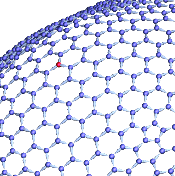
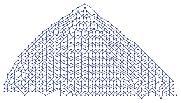
In a layered rendering, this is:

curvedDirectedGraph[n_, neighborhoodSize_, v_ : 1] := With[{graph = NeighborhoodGraph[ResourceFunction["BuckyballGraph"][n], v, neighborhoodSize]}, With[{center = GraphCenter[graph][[1]]}, {HighlightGraph[ Graph3D[Select[ Reap[BreadthFirstScan[graph, center, {"VisitedVertex" -> (Sow[#1 -> #2] &)}]][[2, 1]], #[[1]] != #[[2]] &], DirectedEdges -> True], center], center, ResourceFunction["GraphNeighborhoodVolumes"][ graph, {center}][[1]]}]]; LayeredGraphPlot[First[curvedDirectedGraph[7, 25]], VertexStyle -> ResourceFunction["WolframPhysicsProjectStyleData"]["SpatialGraph", "VertexStyle"], EdgeStyle -> ResourceFunction["WolframPhysicsProjectStyleData"]["SpatialGraph", "EdgeLineStyle"]]

Once again, we can compute the log differences of Ct (the similarity of sphere graphs means that using larger versions does not change the result):

ListLinePlot[ ResourceFunction["LogDifferences"][{1, 4, 10, 19, 31, 46, 64, 85, 109, 136, 166, 197, 231, 266, 304, 342, 383, 424, 468, 512, 558, 604, 652, 700, 748, 796}], PlotRange -> {0, Automatic}, Frame -> True, PlotStyle -> ResourceFunction["WolframPhysicsProjectStyleData"][ "GenericLinePlot", "PlotStyles"]]

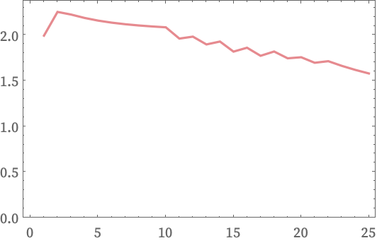
The systematic deviation from the d = 2 result islike in the hypergraph casea reflection of curvature.