Typical Forms of Branchial Graphs: Wolfram Physics Project Technical Background

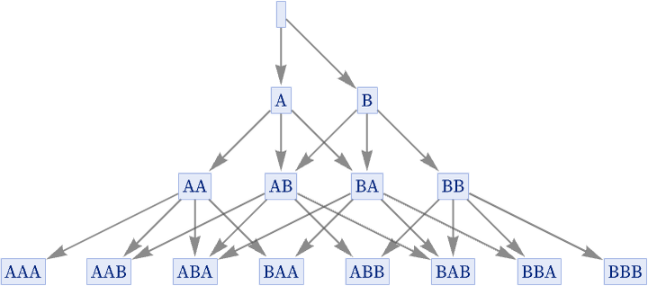
As a first example, consider the (causal invariant) rule which effectively just creates either A or B from nothing:

{"" -> "A", "" -> "B"}

At step t, this rule produces all 2^t possible strings. Its multiway way graph is:

ResourceFunction["MultiwaySystem"][{"" -> "A", "" -> "B"}, "", 3, "StatesGraph", GraphLayout -> "LayeredDigraphEmbedding"]

The succession of branchial graphs is then:

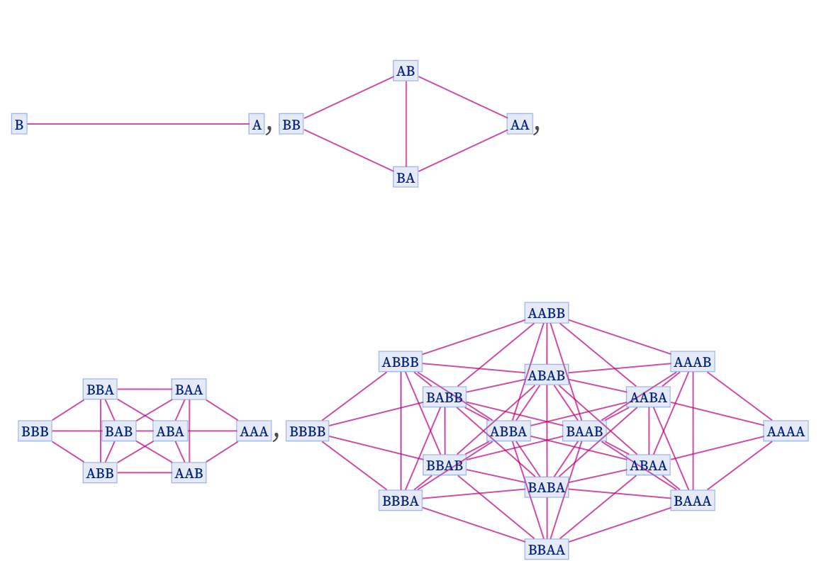
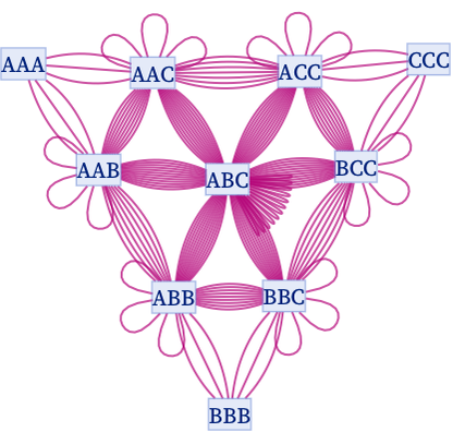
Table[ResourceFunction["MultiwaySystem"][{"" -> "A", "" -> "B"}, "", t, "BranchialGraph"], {t, 4}]

The graph on step t has 2^t nodes and 2^t–2 (t² – t + 4) – 1 edges. The distance on the graph between two states is precisely the difference in the total number of As (or Bs) between them, plus 1—so combining states which differ only through ordering of A and B the last graph becomes:

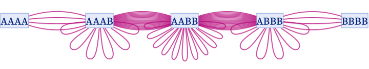
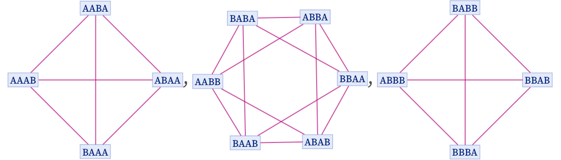
stripMetadata[expression_] := If[Head[expression] === Rule, Last[expression], expression] Graph[{"AAAA" \[UndirectedEdge] "AAAB", "AAAA" \[UndirectedEdge] "AAAB", "AAAA" \[UndirectedEdge] "AAAB", "AAAA" \[UndirectedEdge] "AAAB", "AAAB" \[UndirectedEdge] "AAAB", "AAAB" \[UndirectedEdge] "AABB", "AAAB" \[UndirectedEdge] "AAAB", "AAAB" \[UndirectedEdge] "AABB", "AAAB" \[UndirectedEdge] "AAAB", "AAAB" \[UndirectedEdge] "AABB", "AAAB" \[UndirectedEdge] "AABB", "AAAB" \[UndirectedEdge] "AAAB", "AAAB" \[UndirectedEdge] "AABB", "AAAB" \[UndirectedEdge] "AABB", "AAAB" \[UndirectedEdge] "AAAB", "AAAB" \[UndirectedEdge] "AABB", "AAAB" \[UndirectedEdge] "AABB", "AABB" \[UndirectedEdge] "AABB", "AABB" \[UndirectedEdge] "AABB", "AABB" \[UndirectedEdge] "ABBB", "AABB" \[UndirectedEdge] "AABB", "AABB" \[UndirectedEdge] "ABBB", "AAAB" \[UndirectedEdge] "AABB", "AAAB" \[UndirectedEdge] "AABB", "AAAB" \[UndirectedEdge] "AAAB", "AAAB" \[UndirectedEdge] "AABB", "AAAB" \[UndirectedEdge] "AABB", "AAAB" \[UndirectedEdge] "AABB", "AABB" \[UndirectedEdge] "AABB", "AABB" \[UndirectedEdge] "ABBB", "AABB" \[UndirectedEdge] "AABB", "AABB" \[UndirectedEdge] "AABB", "AABB" \[UndirectedEdge] "ABBB", "AABB" \[UndirectedEdge] "ABBB", "AABB" \[UndirectedEdge] "ABBB", "AABB" \[UndirectedEdge] "AABB", "AABB" \[UndirectedEdge] "ABBB", "AABB" \[UndirectedEdge] "AABB", "AABB" \[UndirectedEdge] "ABBB", "AABB" \[UndirectedEdge] "ABBB", "ABBB" \[UndirectedEdge] "ABBB", "ABBB" \[UndirectedEdge] "ABBB", "ABBB" \[UndirectedEdge] "ABBB", "ABBB" \[UndirectedEdge] "BBBB", "AAAB" \[UndirectedEdge] "AABB", "AAAB" \[UndirectedEdge] "AABB", "AAAB" \[UndirectedEdge] "AABB", "AABB" \[UndirectedEdge] "AABB", "AABB" \[UndirectedEdge] "ABBB", "AABB" \[UndirectedEdge] "AABB", "AABB" \[UndirectedEdge] "ABBB", "AABB" \[UndirectedEdge] "ABBB", "AABB" \[UndirectedEdge] "AABB", "AABB" \[UndirectedEdge] "ABBB", "AABB" \[UndirectedEdge] "ABBB", "ABBB" \[UndirectedEdge] "ABBB", "ABBB" \[UndirectedEdge] "ABBB", "ABBB" \[UndirectedEdge] "BBBB", "AABB" \[UndirectedEdge] "ABBB", "AABB" \[UndirectedEdge] "ABBB", "ABBB" \[UndirectedEdge] "ABBB", "ABBB" \[UndirectedEdge] "BBBB", "ABBB" \[UndirectedEdge] "BBBB"}, {PerformanceGoal -> "Quality", VertexShapeFunction -> {Text[ \!\(\*FrameBox[\!\(Style[stripMetadata[#2], Hue[0.62, 1, 0.48]]\), Background->Directive[ Opacity[0.2], Hue[0.62, 0.45, 0.87]], FrameMargins->None, FrameStyle->Directive[ Opacity[0.5], Hue[0.62, 0.52, 0.82]], StripOnInput->False]\), #1, {0, 0}] &}}, EdgeStyle -> ResourceFunction["WolframPhysicsProjectStyleData"]["BranchialGraph", "EdgeStyle"]]

With the rule

{"" -> "A", "" -> "B", "" -> "C"}

the sequence of branchial graphs is

Table[ResourceFunction["MultiwaySystem"][{"" -> "A", "" -> "B", "" -> "C"}, "", t, "BranchialGraph"], {t, 3}]

and in the last case combining states which differ only in the order of elements, one gets:

stripMetadata[expression_] := If[Head[expression] === Rule, Last[expression], expression] Graph[Map[StringJoin[Sort[Characters[#]]] &, EdgeList@ResourceFunction["MultiwaySystem"][{"" -> "A", "" -> "B", "" -> "C"}, "", 3, "BranchialGraph"], {-1}], {PerformanceGoal -> "Quality", VertexShapeFunction -> {Text[ \!\(\*FrameBox[\!\(Style[stripMetadata[#2], Hue[0.62, 1, 0.48]]\), Background->Directive[ Opacity[0.2], Hue[0.62, 0.45, 0.87]], FrameMargins->None, FrameStyle->Directive[ Opacity[0.5], Hue[0.62, 0.52, 0.82]], StripOnInput->False]\), #1, {0, 0}] &}}, EdgeStyle -> ResourceFunction["WolframPhysicsProjectStyleData"]["BranchialGraph", "EdgeStyle"]]

Note that no rule involving only As can have a nontrivial branchial graph, since all branch pairs immediately resolve.

Consider now the rule:

{"A" -> "AB"}

As mentioned in 5.4, with initial condition AA this rule gives a multiway graph that corresponds to a 2D grid:

ResourceFunction[ "MultiwaySystem"][{"A" -> "AB"}, "AA", 3, "StatesGraph"]

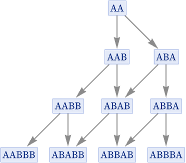
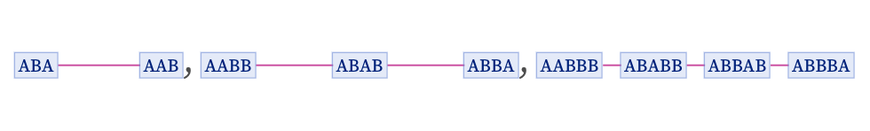
The corresponding branchial graphs are 1D:

Prepend[Table[ ResourceFunction["MultiwaySystem"][{"A" -> "AB"}, "AA", t, "BranchialGraph", ImageSize -> {180, 60}], {t, 2, 3}], ResourceFunction["MultiwaySystem"][{"A" -> "AB"}, "AA", 1, "BranchialGraph", ImageSize -> {Automatic, 60}]]

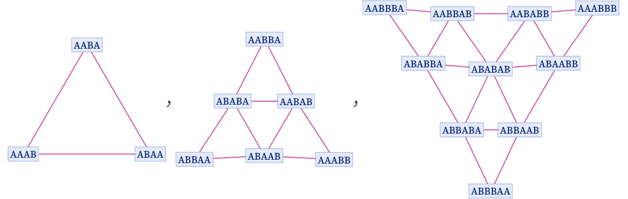
With initial condition AAA, the multiway graph is effectively a 3D grid, and the branchial graph is a 2D grid:

Table[ResourceFunction["MultiwaySystem"][{"A" -> "AB"}, "AAA", t, "BranchialGraph"], {t, 1, 3}]

Some rules produce only finite sequences of branchial graphs. For example, the rule

{"A" -> "B"}

with initial condition AAAA yields what are effectively sections through a cube oriented on its corner:

Table[ResourceFunction["MultiwaySystem"][{"A" -> "B"}, "AAAA", t, "BranchialGraph"], {t, 1, 3}]

As another example producing a finite sequence of branchial graphs, consider the rule:

{"BA" -> "AB"}

Starting from BBBAAA it gives:

Table[ResourceFunction["MultiwaySystem"][{"BA" -> "AB"}, "BBBAAA", t, "BranchialGraph"], {t, 2, 7}]

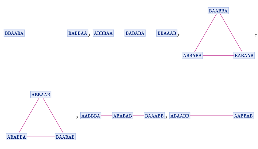
Starting from BBBBBAAAAA it gives:

Table[Graph[ ResourceFunction["MultiwaySystem"][{"BA" -> "AB"}, "BBBBBAAAAA", t, "BranchialGraphStructure"], ImageSize -> 80], {t, 2, 23}]

One can think of this as showing the “shapes” of successive slices through the multiway system for the evolution of this rule.

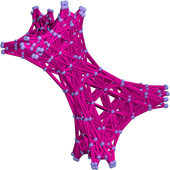
As another example of a rule yielding an infinite sequence of branchial graphs, consider:

{"A" -> "AAB"}

This yields the following branchial graphs:

Table[ResourceFunction["MultiwaySystem"][{"A" -> "AAB"}, "A", t, If[t < 4, "BranchialGraph", "BranchialGraphStructure"]], {t, 2, 6}]

In a 3D rendering, the graph on the next step is:

Graph3D[ResourceFunction["MultiwaySystem"][{"A" -> "AAB"}, "A", 7, "BranchialGraphStructure"]]

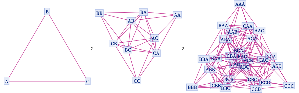
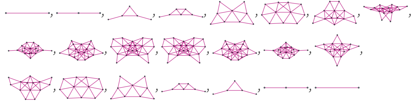
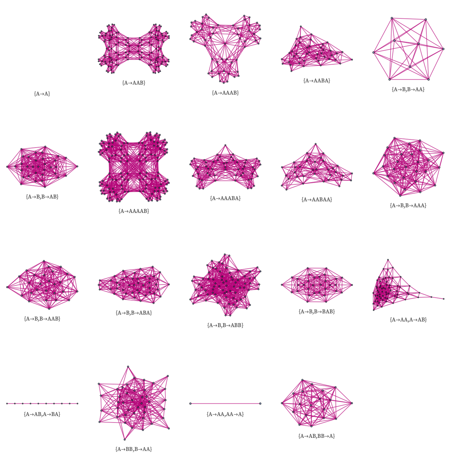
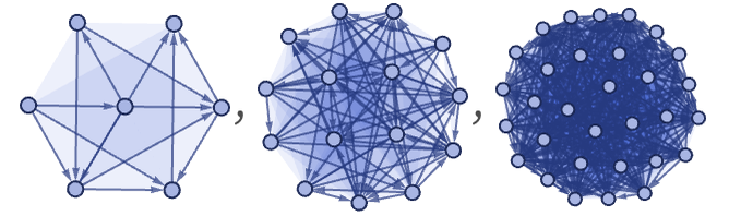
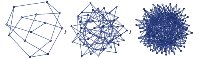
The following are the distinct forms of branchial graphs obtained from rules involving a total of up to 6 As and Bs (starting from a single A):

allrules = {{}, {{"A" -> "A"}, {"A" -> "B"}}, {{"A" -> "AA"}, { "A" -> "AB"}, {"A" -> "BB"}, {"AA" -> "A"}, {"AB" -> "A"}}, {{ "A" -> "AAA"}, {"A" -> "AAB"}, {"A" -> "ABA"}, {"A" -> "ABB"}, { "A" -> "BAB"}, {"A" -> "BBB"}, {"AAA" -> "A"}, {"AAB" -> "A"}, { "AAB" -> "B"}, {"ABA" -> "A"}, {"AA" -> "AA"}, {"AB" -> "AA"}, { "AB" -> "AB"}, {"AB" -> "BA"}, {"A" -> "A", "A" -> "A"}, { "A" -> "A", "A" -> "B"}, {"A" -> "A", "B" -> "A"}, { "A" -> "A", "B" -> "B"}, {"A" -> "B", "A" -> "A"}, { "A" -> "B", "A" -> "B"}, {"A" -> "B", "B" -> "A"}, { "A" -> "B", "B" -> "B"}}, {{"A" -> "AAAA"}, {"A" -> "AAAB"}, { "A" -> "AABA"}, {"A" -> "AABB"}, {"A" -> "ABAB"}, { "A" -> "ABBA"}, {"A" -> "ABBB"}, {"A" -> "BAAB"}, { "A" -> "BABB"}, {"A" -> "BBBB"}, {"AAAA" -> "A"}, { "AAAB" -> "A"}, {"AAAB" -> "B"}, {"AABA" -> "A"}, { "AABB" -> "A"}, {"ABBA" -> "A"}, {"AA" -> "AAA"}, { "AA" -> "ABA"}, {"AB" -> "AAA"}, {"AB" -> "AAB"}, { "AB" -> "ABA"}, {"AB" -> "BAA"}, {"AAA" -> "AA"}, { "AAB" -> "AA"}, {"AAB" -> "AB"}, {"AAB" -> "BA"}, { "AAB" -> "BB"}, {"ABA" -> "AA"}, {"A" -> "A", "A" -> "AA"}, { "A" -> "A", "A" -> "AB"}, {"A" -> "A", "A" -> "BB"}, { "A" -> "A", "B" -> "AA"}, {"A" -> "A", "B" -> "AB"}, { "A" -> "A", "B" -> "BB"}, {"A" -> "B", "B" -> "AA"}, { "A" -> "B", "B" -> "AB"}, {"A" -> "B", "B" -> "BB"}, { "A" -> "A", "AA" -> "A"}, {"A" -> "A", "AA" -> "B"}, { "A" -> "A", "AB" -> "A"}, {"A" -> "A", "AB" -> "B"}, { "A" -> "A", "BB" -> "A"}, {"A" -> "A", "BB" -> "B"}, { "A" -> "B", "BB" -> "A"}, {"A" -> "B", "BB" -> "B"}}, {{ "A" -> "AAAAA"}, {"A" -> "AAAAB"}, {"A" -> "AAABA"}, { "A" -> "AAABB"}, {"A" -> "AABAA"}, {"A" -> "AABAB"}, { "A" -> "AABBA"}, {"A" -> "AABBB"}, {"A" -> "ABAAB"}, { "A" -> "ABABA"}, {"A" -> "ABABB"}, {"A" -> "ABBAB"}, { "A" -> "ABBBA"}, {"A" -> "ABBBB"}, {"A" -> "BAAAB"}, { "A" -> "BAABB"}, {"A" -> "BABAB"}, {"A" -> "BABBB"}, { "A" -> "BBABB"}, {"A" -> "BBBBB"}, {"AAAAA" -> "A"}, { "AAAAB" -> "A"}, {"AAAAB" -> "B"}, {"AAABA" -> "A"}, { "AAABB" -> "A"}, {"AAABB" -> "B"}, {"AABAB" -> "A"}, { "AABAB" -> "B"}, {"AABBA" -> "A"}, {"ABABA" -> "A"}, { "ABBBA" -> "A"}, {"AA" -> "AAAA"}, {"AA" -> "AABA"}, { "AA" -> "ABBA"}, {"AB" -> "AAAA"}, {"AB" -> "AAAB"}, { "AB" -> "AABA"}, {"AB" -> "AABB"}, {"AB" -> "ABAA"}, { "AB" -> "ABAB"}, {"AB" -> "ABBA"}, {"AB" -> "BAAA"}, { "AB" -> "BABA"}, {"AB" -> "BBAA"}, {"AAAA" -> "AA"}, { "AAAB" -> "AA"}, {"AAAB" -> "AB"}, {"AAAB" -> "BA"}, { "AAAB" -> "BB"}, {"AABA" -> "AA"}, {"AABB" -> "AA"}, { "AABB" -> "AB"}, {"AABB" -> "BA"}, {"ABAB" -> "AB"}, { "ABBA" -> "AA"}, {"AAA" -> "AAA"}, {"AAB" -> "AAA"}, { "AAB" -> "AAB"}, {"AAB" -> "ABA"}, {"AAB" -> "ABB"}, { "AAB" -> "BAA"}, {"AAB" -> "BAB"}, {"AAB" -> "BBA"}, { "AAB" -> "BBB"}, {"ABA" -> "AAA"}, {"ABA" -> "ABA"}, { "A" -> "A", "A" -> "AAA"}, {"A" -> "A", "A" -> "AAB"}, { "A" -> "A", "A" -> "ABA"}, {"A" -> "A", "A" -> "ABB"}, { "A" -> "A", "A" -> "BAB"}, {"A" -> "A", "A" -> "BBB"}, { "A" -> "A", "B" -> "AAA"}, {"A" -> "A", "B" -> "AAB"}, { "A" -> "A", "B" -> "ABA"}, {"A" -> "A", "B" -> "ABB"}, { "A" -> "A", "B" -> "BAB"}, {"A" -> "A", "B" -> "BBB"}, { "A" -> "B", "B" -> "AAA"}, {"A" -> "B", "B" -> "AAB"}, { "A" -> "B", "B" -> "ABA"}, {"A" -> "B", "B" -> "ABB"}, { "A" -> "B", "B" -> "BAB"}, {"A" -> "B", "B" -> "BBB"}, { "A" -> "A", "AAA" -> "A"}, {"A" -> "A", "AAA" -> "B"}, { "A" -> "A", "AAB" -> "A"}, {"A" -> "A", "AAB" -> "B"}, { "A" -> "A", "ABA" -> "A"}, {"A" -> "A", "ABA" -> "B"}, { "A" -> "A", "ABB" -> "A"}, {"A" -> "A", "ABB" -> "B"}, { "A" -> "A", "BAB" -> "A"}, {"A" -> "A", "BAB" -> "B"}, { "A" -> "A", "BBB" -> "A"}, {"A" -> "A", "BBB" -> "B"}, { "A" -> "B", "BBB" -> "A"}, {"A" -> "B", "BBB" -> "B"}, { "A" -> "A", "AA" -> "AA"}, {"A" -> "A", "AA" -> "AB"}, { "A" -> "A", "AA" -> "BB"}, {"A" -> "A", "AB" -> "AA"}, { "A" -> "A", "AB" -> "AB"}, {"A" -> "A", "AB" -> "BA"}, { "A" -> "A", "AB" -> "BB"}, {"A" -> "A", "BB" -> "AA"}, { "A" -> "A", "BB" -> "AB"}, {"A" -> "A", "BB" -> "BB"}, { "A" -> "B", "AA" -> "AA"}, {"A" -> "B", "AA" -> "AB"}, { "A" -> "B", "AA" -> "BB"}, {"A" -> "B", "AB" -> "AA"}, { "A" -> "B", "AB" -> "AB"}, {"A" -> "B", "AB" -> "BA"}, { "A" -> "B", "AB" -> "BB"}, {"A" -> "B", "BB" -> "AA"}, { "A" -> "B", "BB" -> "AB"}, {"A" -> "B", "BB" -> "BB"}, { "A" -> "AA", "A" -> "AA"}, {"A" -> "AA", "A" -> "AB"}, { "A" -> "AA", "B" -> "AA"}, {"A" -> "AA", "B" -> "AB"}, { "A" -> "AA", "B" -> "BB"}, {"A" -> "AB", "A" -> "AA"}, { "A" -> "AB", "A" -> "AB"}, {"A" -> "AB", "A" -> "BA"}, { "A" -> "AB", "B" -> "AA"}, {"A" -> "AB", "B" -> "AB"}, { "A" -> "AB", "B" -> "BA"}, {"A" -> "AB", "B" -> "BB"}, { "A" -> "BB", "A" -> "BB"}, {"A" -> "BB", "B" -> "AA"}, { "A" -> "BB", "B" -> "AB"}, {"A" -> "BB", "B" -> "BB"}, { "A" -> "AA", "AA" -> "A"}, {"A" -> "AA", "AB" -> "A"}, { "A" -> "AA", "AB" -> "B"}, {"A" -> "AA", "BB" -> "A"}, { "A" -> "AA", "BB" -> "B"}, {"A" -> "AB", "AB" -> "A"}, { "A" -> "AB", "BA" -> "A"}, {"A" -> "AB", "BB" -> "A"}, { "A" -> "AB", "BB" -> "B"}, {"A" -> "BB", "BB" -> "A"}, { "A" -> "BB", "BB" -> "B"}, {"AA" -> "A", "AA" -> "A"}, { "AA" -> "A", "AB" -> "A"}, {"AA" -> "A", "AB" -> "B"}, { "AA" -> "A", "BB" -> "A"}, {"AA" -> "A", "BB" -> "B"}, { "AA" -> "B", "BB" -> "A"}, {"AA" -> "B", "BB" -> "B"}, { "AB" -> "A", "AA" -> "A"}, {"AB" -> "A", "AB" -> "A"}, { "AB" -> "A", "BA" -> "A"}, {"AB" -> "A", "BB" -> "B"}, { "A" -> "A", "A" -> "A", "A" -> "A"}, { "A" -> "A", "A" -> "A", "A" -> "B"}, { "A" -> "A", "A" -> "A", "B" -> "A"}, { "A" -> "A", "A" -> "A", "B" -> "B"}, { "A" -> "A", "A" -> "B", "A" -> "A"}, { "A" -> "A", "A" -> "B", "A" -> "B"}, { "A" -> "A", "A" -> "B", "B" -> "A"}, { "A" -> "A", "A" -> "B", "B" -> "B"}, { "A" -> "A", "B" -> "A", "A" -> "A"}, { "A" -> "A", "B" -> "A", "A" -> "B"}, { "A" -> "A", "B" -> "A", "B" -> "A"}, { "A" -> "A", "B" -> "A", "B" -> "B"}, { "A" -> "A", "B" -> "B", "A" -> "A"}, { "A" -> "A", "B" -> "B", "A" -> "B"}, { "A" -> "A", "B" -> "B", "B" -> "A"}, { "A" -> "A", "B" -> "B", "B" -> "B"}, { "A" -> "B", "A" -> "A", "A" -> "A"}, { "A" -> "B", "A" -> "A", "A" -> "B"}, { "A" -> "B", "A" -> "A", "B" -> "A"}, { "A" -> "B", "A" -> "A", "B" -> "B"}, { "A" -> "B", "A" -> "B", "A" -> "A"}, { "A" -> "B", "A" -> "B", "A" -> "B"}, { "A" -> "B", "A" -> "B", "B" -> "A"}, { "A" -> "B", "A" -> "B", "B" -> "B"}, { "A" -> "B", "B" -> "A", "A" -> "A"}, { "A" -> "B", "B" -> "A", "A" -> "B"}, { "A" -> "B", "B" -> "A", "B" -> "A"}, { "A" -> "B", "B" -> "A", "B" -> "B"}, { "A" -> "B", "B" -> "B", "A" -> "A"}, { "A" -> "B", "B" -> "B", "A" -> "B"}, { "A" -> "B", "B" -> "B", "B" -> "A"}, { "A" -> "B", "B" -> "B", "B" -> "B"}}}; GraphicsGrid[ Partition[ Labeled[Graph[First[#], ImageSize -> {120, Automatic}], Text[Style[Last[#], Small], BaseStyle -> {GrayLevel[.25], FontSize -> .95 Inherited, FontFamily -> "Source Serif Pro"}]] & /@ (First /@ Gather[ParallelMap[ Catch[Module[{u}, Do[u = ResourceFunction["MultiwaySystem"][#, "A", t, "BranchialGraphStructure"]; If[VertexCount[u] > 150 || EdgeCount[u] > 150, Throw[u]], {t, 9}]; u]] -> # &, Catenate[allrules]], IsomorphicGraphQ[First[#], First[#2]] &]), UpTo[5]], ImageSize -> Full]

We have seen that branchial graphs can form regular grids. But many branchial graphs have much higher levels of connectivity. No branchial graph can continue to be a complete graph (with all neighbors having distance 1) for more than a limited number of steps. However, the diameters of branchial graphs do tend to grow slowly, and on step t they can be no larger than t. Some branchial graphs show linear or polynomial growth with the number of steps in vertex and edge count, but many show exponential growth.

In analogy to what we did for hypergraphs and causal graphs, we can define a quantity B_b which measures the number of nodes in the branchial graph reached by going out to graph distance b from a given node.

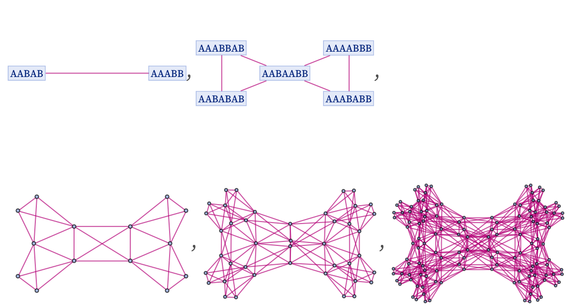
Consider for example the rule:

{"" -> "A", "" -> "B"}

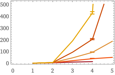
The sequence of forms for B_b as a function of b on successive steps is:

(* data=ParallelTable[With[{q=ResourceFunction["MultiwaySystem"][{""\ ->"A",""->"B"},"A",t,"BranchialGraphStructure"]},\ ResourceFunction["RaggedMeanAround"][Values[ResourceFunction[\ "GraphNeighborhoodVolumes"][q]]]],{t,2,10}];*) data = {{1, Around[5.285714285714286, 0.4738035414793428], 7}, {1, Around[8.466666666666667, 0.5679257720333551], Around[14.2, 0.29600514796038196`], 15}, {1, Around[12.612903225806452`, 0.5932912018776778], Around[26.677419354838708`, 0.6432228944833299], Around[30.5, 0.20249763209798527`], 31}, {1, Around[17.73015873015873, 0.5712009559758332], Around[47.76190476190476, 1.0489099712853804`], Around[60.20634920634921, 0.5145893675380103], Around[62.567567567567565`, 0.17984202502411828`], 63}, {1, Around[23.818897637795274`, 0.5229894603215057], Around[82.02362204724409, 1.4934119612335364`], Around[115.92913385826772`, 1.0479791769166356`], Around[125.08547008547009`, 0.3728900064459459], Around[126.61702127659575`, 0.16252286963346457`], 127}, {1, Around[30.88235294117647, 0.46332984985248293`], Around[135.48627450980393`, 1.9461156427121906`], Around[218.85098039215686`, 1.8325886058313723`], Around[247.3686274509804, 0.8073820767213228], Around[253.3151515151515, 0.3284722481171782], Around[254.6551724137931, 0.1487022387199374], 255}, {1, Around[38.92563600782779, 0.40076465690870194`], Around[215.67710371819962`, 2.368485227967195], Around[404.6908023483366, 2.9189051834643434`], Around[484.174168297456, 1.5993930142316763`], Around[505.50840336134456`, 0.5946948358202185], Around[509.49107142857144`, 0.29312476541588733`], Around[510.6857142857143, 0.13732562011173036`], 511}, {1, Around[47.95405669599218, 0.3400904972754984], Around[331.6099706744868, 2.7244825572310134`], Around[731.4183773216031, 4.344517555886898], Around[938.8044965786901, 2.8726749708313584`], Around[1003.8152492668622`, 1.2037711299323357`], Around[1018.1155492154065`, 0.5216323873097088], Around[1021.6305084745762`, 0.2645669690687118], Around[1022.710843373494, 0.1277418887852933], 1023}, {1, Around[57.97215437225208, 0.2839861353523077], Around[493.80410356619444`, 2.988641002117058], Around[1289.3849535906204`, 6.115580447758085], Around[1800.6717147044455`, 4.828132424729713], Around[1983.4406448461164`, 2.343776770006537], Around[2032.7667881311818`, 0.8929438944650846], Around[2042.5967903711132`, 0.4624503929791409], Around[2045.7440633245383`, 0.2411067638473127], Around[2046.7319587628865`, 0.11952391951504247`], 2047}, {1, Around[68.98339438339438, 0.23384832731738137`], Around[714.2830280830281, 3.148790166334143], Around[2213.9103785103785`, 8.192951954277284], Around[3409.294017094017, 7.716372799712135], Around[3900.0251526251527`, 4.258705958057957], Around[4048.425152625153, 1.7420753937278297`], Around[4082.2572798903734`, 0.7804699528669187], Around[4090.9869281045753`, 0.41420446234635594`], Around[4093.83857442348, 0.2215287128706958], Around[4094.75, 0.11237748942159248`], 4095}}; ListLinePlot[data, Frame -> True, PlotStyle -> ResourceFunction["WolframPhysicsProjectStyleData"][ "GenericLinePlot", "PlotStyles"]]

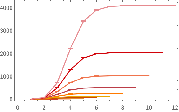
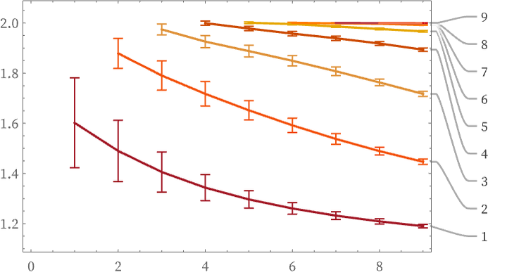
At step t, the diameter of the graph is just t, and B_b=t = 2^t. For smaller b, the ratios of the B_b for given b at successive steps t steadily decrease, perhaps suggesting ultimately less-than-exponential growth:

data = {{1, Around[5.285714285714286, 0.4738035414793428], 7}, {1, Around[8.466666666666667, 0.5679257720333551], Around[14.2, 0.29600514796038196`], 15}, {1, Around[12.612903225806452`, 0.5932912018776778], Around[26.677419354838708`, 0.6432228944833299], Around[30.5, 0.20249763209798527`], 31}, {1, Around[17.73015873015873, 0.5712009559758332], Around[47.76190476190476, 1.0489099712853804`], Around[60.20634920634921, 0.5145893675380103], Around[62.567567567567565`, 0.17984202502411828`], 63}, {1, Around[23.818897637795274`, 0.5229894603215057], Around[82.02362204724409, 1.4934119612335364`], Around[115.92913385826772`, 1.0479791769166356`], Around[125.08547008547009`, 0.3728900064459459], Around[126.61702127659575`, 0.16252286963346457`], 127}, {1, Around[30.88235294117647, 0.46332984985248293`], Around[135.48627450980393`, 1.9461156427121906`], Around[218.85098039215686`, 1.8325886058313723`], Around[247.3686274509804, 0.8073820767213228], Around[253.3151515151515, 0.3284722481171782], Around[254.6551724137931, 0.1487022387199374], 255}, {1, Around[38.92563600782779, 0.40076465690870194`], Around[215.67710371819962`, 2.368485227967195], Around[404.6908023483366, 2.9189051834643434`], Around[484.174168297456, 1.5993930142316763`], Around[505.50840336134456`, 0.5946948358202185], Around[509.49107142857144`, 0.29312476541588733`], Around[510.6857142857143, 0.13732562011173036`], 511}, {1, Around[47.95405669599218, 0.3400904972754984], Around[331.6099706744868, 2.7244825572310134`], Around[731.4183773216031, 4.344517555886898], Around[938.8044965786901, 2.8726749708313584`], Around[1003.8152492668622`, 1.2037711299323357`], Around[1018.1155492154065`, 0.5216323873097088], Around[1021.6305084745762`, 0.2645669690687118], Around[1022.710843373494, 0.1277418887852933], 1023}, {1, Around[57.97215437225208, 0.2839861353523077], Around[493.80410356619444`, 2.988641002117058], Around[1289.3849535906204`, 6.115580447758085], Around[1800.6717147044455`, 4.828132424729713], Around[1983.4406448461164`, 2.343776770006537], Around[2032.7667881311818`, 0.8929438944650846], Around[2042.5967903711132`, 0.4624503929791409], Around[2045.7440633245383`, 0.2411067638473127], Around[2046.7319587628865`, 0.11952391951504247`], 2047}, {1, Around[68.98339438339438, 0.23384832731738137`], Around[714.2830280830281, 3.148790166334143], Around[2213.9103785103785`, 8.192951954277284], Around[3409.294017094017, 7.716372799712135], Around[3900.0251526251527`, 4.258705958057957], Around[4048.425152625153, 1.7420753937278297`], Around[4082.2572798903734`, 0.7804699528669187], Around[4090.9869281045753`, 0.41420446234635594`], Around[4093.83857442348, 0.2215287128706958], Around[4094.75, 0.11237748942159248`], 4095}}; ListLinePlot[ Most[MapIndexed[ Callout[Drop[#, First[#2] - 1], Style[First[#2], GrayLevel[.25], FontSize -> .95 Inherited, FontFamily -> "Source Serif Pro"]] &, MapIndexed[{#2[[2]], #1} &, Take[Ratios /@ Transpose[PadRight[data, Automatic, None]], {2, -2}], {2}]]], Frame -> True, PlotStyle -> ResourceFunction["WolframPhysicsProjectStyleData"][ "GenericLinePlot", "PlotStyles"]]

One can ask what the limit of a branchial graph after a large number of steps may be. As an initial possible model, consider graphs representing n-cubes in progressively higher dimensions:

Table[GridGraph[Table[2, n], ImageSize -> Tiny, VertexStyle -> ResourceFunction["WolframPhysicsProjectStyleData"]["SpatialGraph", "VertexStyle"], EdgeStyle -> ResourceFunction["WolframPhysicsProjectStyleData"]["SpatialGraph", "EdgeLineStyle"]], {n, 6}]

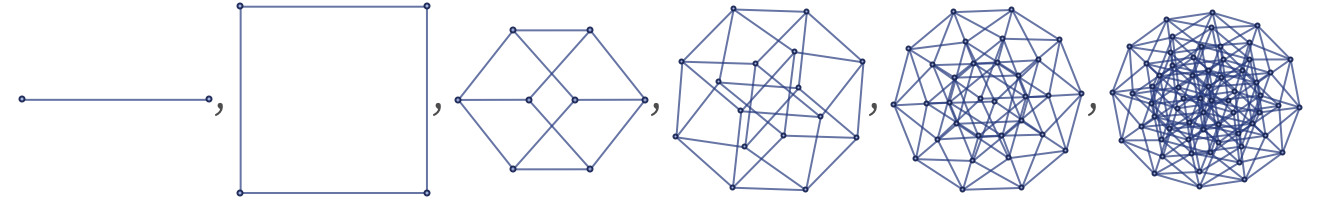
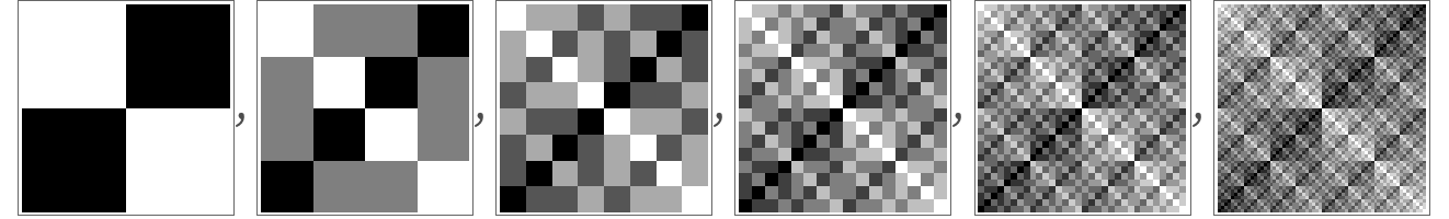
The graph distances between nodes in these graphs are exactly the same as the Euclidean distances between the 2ⁿ possible tuples of 0s and 1s (here shown in distance matrices arranged in lexicographic order):

Table[ArrayPlot[ DistanceMatrix[Tuples[{0, 1}, n], DistanceFunction -> (Norm[#1 - #2]^2 &)], ImageSize -> Tiny], {n, 1, 6}]

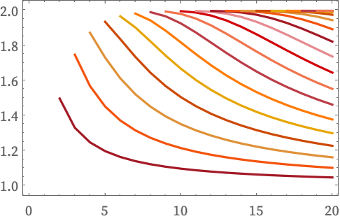
The values of B_b in this case can be found from [11:A008949]:

ListLinePlot[ Accumulate /@ Table[Binomial[n, i], {n, 0, 10}, {i, 0, n}], Frame -> True, PlotStyle -> ResourceFunction["WolframPhysicsProjectStyleData"][ "GenericLinePlot", "PlotStyles"]]

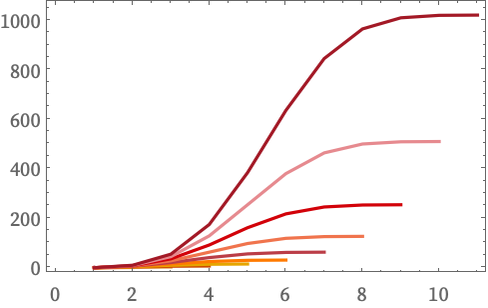
This shows the ratios of B_bfor given b for successive n:

With[{data = Accumulate /@ Table[Binomial[n, i], {n, 0, 20}, {i, 0, n}]}, ListLinePlot[ Most[MapIndexed[Drop[#, First[#2] - 1] &, MapIndexed[{#2[[2]], #1} &, Take[Ratios /@ Transpose[PadRight[data, Automatic, None]], {2, -2}], {2}]]], Frame -> True, PlotStyle -> ResourceFunction["WolframPhysicsProjectStyleData"][ "GenericLinePlot", "PlotStyles"]]]

Much as one can consider progressively larger grid graphs as limiting to a manifold, so perhaps one may consider higher and higher “dimensional” cube graphs as limiting to a Hilbert space.

It is also conceivable that limits of branchial graphs may be related to projective spaces [78]. As one potential connection, one can look at discrete models of incidence geometry [79]. For example, with integers representing points and triples representing lines, the Fano plane

Select[Subsets[Range[2^3 - 1], {3}], BitXor @@ # == 0 &]

is a discrete model of the projective plane. One can consider the sequence of such objects as hypergraphs

Table[ResourceFunction["WolframModelPlot"][ Select[Subsets[Range[2^n - 1], {3}], BitXor @@ # == 0 &], ImageSize -> Tiny], {n, 3, 5}]

and representing both points and lines here as nodes, these correspond to the graphs:

Table[Graph[ UndirectedEdge @@@ Flatten[Table[{k, #} & /@ Select[Select[Subsets[Range[2^n - 1], {3}], BitXor @@ # == 0 &], MemberQ[#, k] &], {k, 1, 2^n - 1}], 1], ImageSize -> Tiny, VertexStyle -> ResourceFunction["WolframPhysicsProjectStyleData"]["SpatialGraph", "VertexStyle"], EdgeStyle -> ResourceFunction["WolframPhysicsProjectStyleData"]["SpatialGraph", "EdgeLineStyle"]], {n, 3, 5}]

But for such graphs one finds that B_b has a very different form from typical branchial graphs:

ListLinePlot[{{1, 4, 10, 14}, {1, Around[5.2, 0.26186146828319085`], 22, Around[38.8, 1.0474458731327634`], 50}, {1, Around[ 6., 0.3287979746107146], 46, Around[ 92.66666666666667, 3.0687810963666697`], 186}, {1, Around[ 6.470588235294118, 0.2974238723295474], 94, Around[ 203.41176470588235`, 5.948477446590948], 714}, {1, Around[ 6.7272727272727275`, 0.2364845371429418], 190, Around[ 426.72727272727275`, 9.774694201908261], 2794}}, Frame -> True, PlotStyle -> ResourceFunction["WolframPhysicsProjectStyleData"][ "GenericLinePlot", "PlotStyles"]]

An alternative approach to connecting with discrete models of projective space is to think in terms of lattice theory [69][80][81]. A multiway graph can be interpreted as a lattice (in the algebraic sense), with its evolution defining the partial order in the lattice. The states in the multiway system are elements in the lattice, and the meet and join operations in the lattice correspond to finding the common ancestors and common successors of states.

The analogy with projective geometry is based on thinking of states in the multiway system (which correspond to elements in the lattice) as points, connected by lines that correspond to their evolution in the multiway system. Points are considered collinear if they have the same common successor. But (assuming the multiway system starts from a single state), causal invariance is exactly the condition that any set of points will eventually have a common successor—or in other words, that all lines will eventually intersect, suggesting that the multiway graph is indeed in some sense a discrete model of projective space—so that branchial graphs may also be models of projective Hilbert spaces.

A Class of Models with the Potential to Represent Fundamental Physics

5.16 Typical Forms of Branchial Graphs