5.15 The Concept of Branchial Graphs

Causal graphs provide one kind of summary of the evolution of a system, based on capturing the causal relationships between events. What we call branchial graphs provide another kind of summary, based on capturing relationships between states on different branches of a multiway system. And whereas causal graphs capture relationships between events at different steps in the evolution of a system, branchial graphs capture relationships between states on different branches at a given step. And in a sense they define a map for exploring branchial space in a multiway system.

One might perhaps have imagined that states on different branches of a multiway system would be completely independent. But when causal invariance is present they are definitely not—because for example whenever they split (to form a branch pair), they will always merge again.

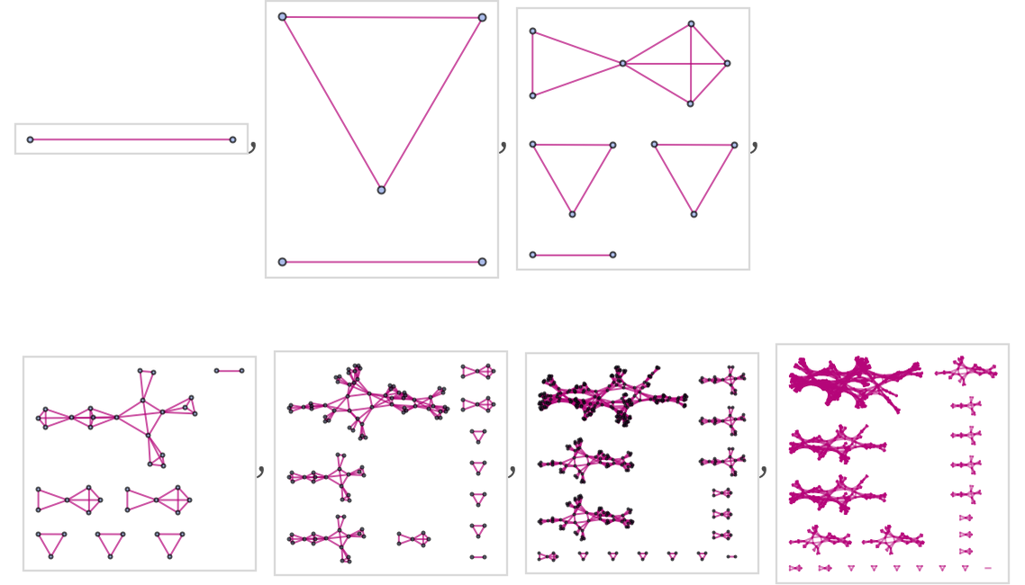
Consider the multiway evolution graph (for the rule {A  AB, B  A}):

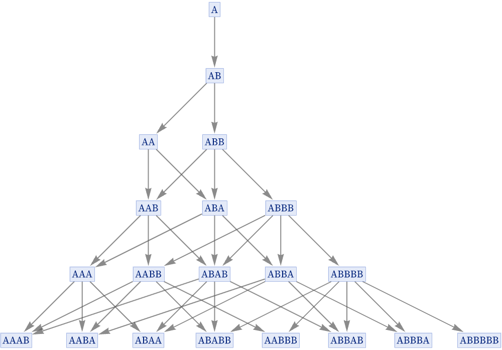
Look at the second-to-last step shown. This contains the following unresolved branch pairs:

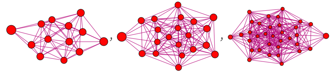
The two states in each of these branch pairs are related, in the sense that they diverged from a common ancestor—and will converge to a common successor. We form the branchial graph by connecting the states that appear in newly unresolved branch pairs at a given step. For the steps shown in the evolution graph above, the successive branchial graphs are:

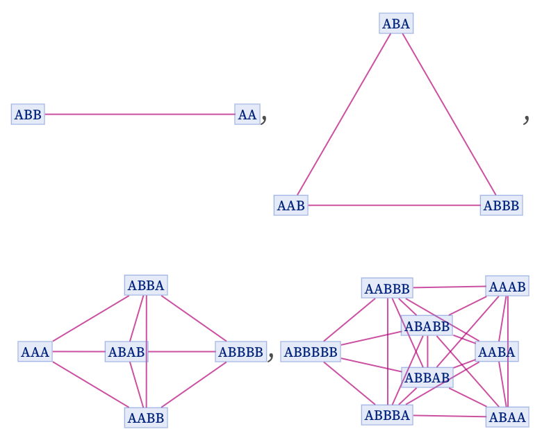
For the next few steps, the states’ branchial graphs are:

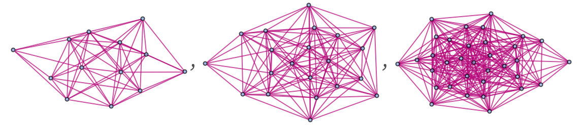
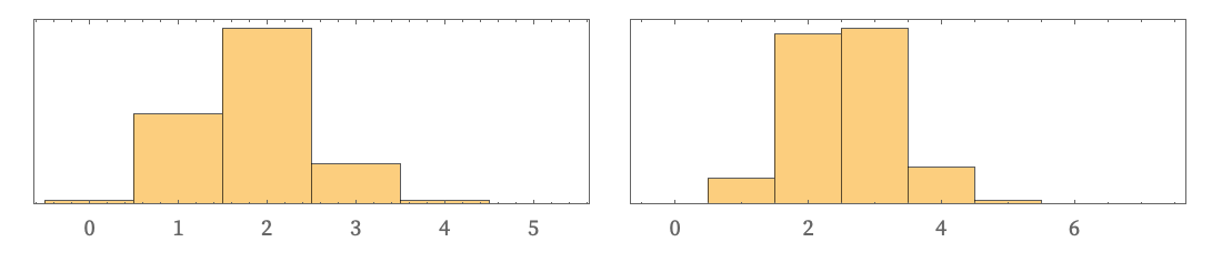
For the rule shown here, the number of nodes at the t^th step is the t^th Fibonacci number, or ∼ϕ^t for large t. The graphs are highly connected, but far from completely so. The number of edges ~ 2^t, while the diameter is . The degree of transitivity (i.e. whether X being connected to Y and Y being connected Z implies X being connected to Z) [76] gradually decreases with t. As a measure of uniformity, one can look at the local clustering coefficient [77] (which measures to what extent there are local complete graphs):

The graphs have somewhat complex vertex degree distributions (here shown after 10 and 15 steps):

For the rule we are showing here, the branchial graph turns out to have a particularly simple interpretation as a map of the level of common ancestry of states. By definition, if two states are directly connected on the branchial graph, it means they had an immediate common ancestor one step before. But what does it mean if two states are graph distance 2 apart?

The particular rule shown here has the property that it is causal invariant, but also that all branch pairs resolve in just one step. And from this it follows that states that are distance 2 apart on the branchial graph must have a common ancestor 2 steps back. And in general the distance on the branchial graph is equal to the number of steps one must go back before one gets to a common ancestor.

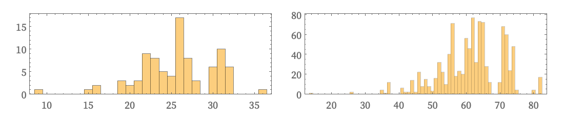
The following histograms show the distribution of graph distances between all pairs of states at steps 10 and 15—or alternatively, the distribution of how many steps it has been since the states had a common ancestor (for this rule the mean increases roughly like ):

We are defining the branchial graph to be based on looking at branch pairs that are unresolved at a particular step, and are new at that step. But we could generalize to consider a “thickened” branchial graph that includes all branch pairs that have been new within the past m steps. By doing this we can capture common ancestry of states even when they are associated with branch pairs that take up to m steps to resolve—but when we do this it is at the cost of having many additions to the graph associated with branch pairs that have “come and gone” within our thickening depth.

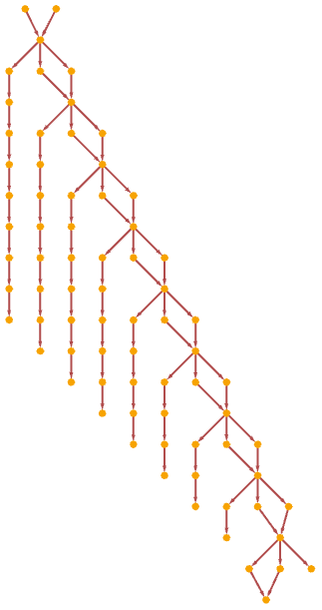
It should be noted that any possible interpretation of branchial graphs in terms of common ancestors depends on having causal invariance. Absent causal invariance, there is no guarantee that states with common ancestors will even be connected in the branchial graph. As an extreme example, consider the rule:

The multiway graph for this rule is a tree

and its branchial graph on successive steps just consists of a collection of disconnected pieces:

By thickening the branchial graph by m steps, one could capture m steps of common ancestry. And in general one could imagine infinitely thickening the graph, so that one looks all the way back to the initial conditions. But the branchial graph one would get in this way would essentially just be a copy of the whole multiway graph.

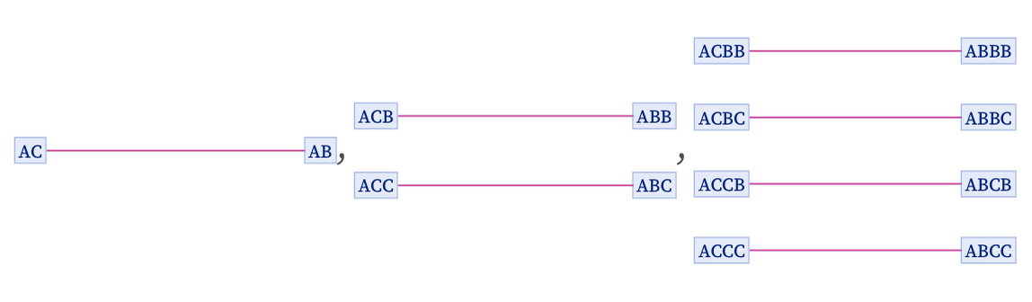
When a rule has branch pairs that take several steps to resolve, it is possible for the branchial graph to be disconnected, even when the rule is causal invariant. Consider for example the rule

in which the branch pair {BAAB, BBABB} takes 3 steps to resolve. The first few branchial graphs for this rule are:

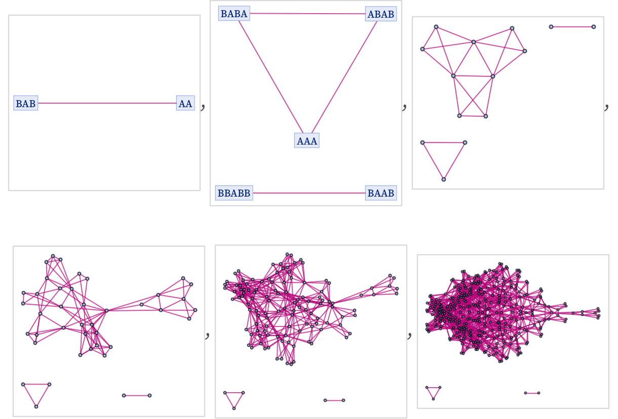
It is fairly common to get branchial graphs in which a few disconnected pieces are “thrown off” in the first few steps, and never recombine. Sometimes, however, disconnected pieces can recombine. The rule

starting from initial condition A yields the sequence of branchial graphs:

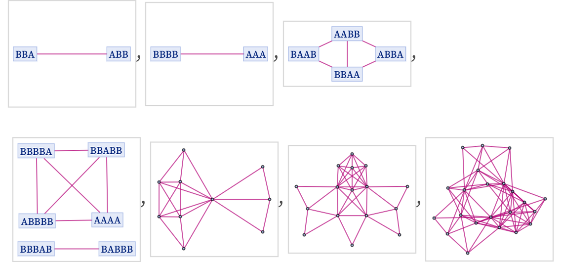
Sometimes the branchial graph can break into many components. This happens for the rule

starting from initial condition AA:

The causal graph for this rule reveals that there is also causal disconnection in this case: