A Class of Models with the Potential to Represent Fundamental Physics
  1. Introduction
  2. Basic Form of Models
  3. Typical Behaviors
  4. Limiting Behavior and Emergent Geometry
  5. The Updating Process for String Substitution Systems
  6. The Updating Process in Our Models
  7. Equivalence and Computation in Our Models
  8. Potential Relation to Physics
  9. Additional Material
  10. References
  11. Index

6.11 Global Symmetries and Conservation Laws

Given the rule (stated here using numbers rather than our usual letters)

{{1, 2, 3}, {3, 4, 5}} -> {{6, 7, 1}, {6, 3, 8}, {5, 7, 8}}

if we reverse the elements in each relation we get:

ApplyPerm[perm_, rule_] := Map[#[[perm]] &, #, {2}] &@rule; ApplyPerm[{3, 2, 1}, {{1, 2, 3}, {3, 4, 5}} -> {{6, 7, 1}, {6, 3, 8}, {5, 7, 8}}]

But the canonical version of this rule is:

ApplyPerm[perm_, rule_] := Map[#[[perm]] &, #, {2}] &@rule; ResourceFunction["CanonicalWolframModelRule"][ ApplyPerm[{3, 2, 1}, {{1, 2, 3}, {3, 4, 5}} -> {{6, 7, 1}, {6, 3, 8}, {5, 7, 8}}]]

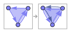
In graphical form, the rule and its transform are:

ApplyPerm[perm_, rule_] := Map[#[[perm]] &, #, {2}] &@rule; RulePlot[ResourceFunction["WolframModel"][#], VertexLabels -> Automatic, ImageSize -> 300] & /@ {#, ApplyPerm[{3, 2, 1}, #]} &[{{1, 2, 3}, {3, 4, 5}} -> {{6, 7, 1}, {6, 3, 8}, {5, 7, 8}}]

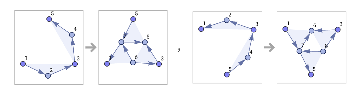
Most rules would not be left invariant under a reversal of each relation. For example, the rule

{{1, 2, 3}, {2, 4, 5}} -> {{5, 6, 4}, {6, 5, 3}, {7, 8, 5}}

yields after reversal of each relation

ApplyPerm[perm_, rule_] := Map[#[[perm]] &, #, {2}] &@rule; ApplyPerm[{3, 2, 1}, {{1, 2, 3}, {2, 4, 5}} -> {{5, 6, 4}, {6, 5, 3}, {7, 8, 5}}]

but the canonical form of this is

ApplyPerm[perm_, rule_] := Map[#[[perm]] &, #, {2}] &@rule; ResourceFunction["CanonicalWolframModelRule"][ ApplyPerm[{3, 2, 1}, {{1, 2, 3}, {2, 4, 5}} -> {{5, 6, 4}, {6, 5, 3}, {7, 8, 5}}]]

which is not the same as the original rule.

If a rule is invariant under a symmetry operation such as reversing each relation, it implies that the rule commutes with the symmetry operation. So given a rule R and a symmetry operation Θ, this means that for any state S, R (Θ S) must be the same as Θ (R S).

With the symmetric rule above, evolving from a particular initial state gives:

h0 = {{1, 2, 3}, {2, 3, 4}, {3, 1, 4}}; ResourceFunction[ "WolframModel"][{{1, 2, 3}, {3, 4, 5}} -> {{6, 7, 1}, {6, 3, 8}, {5, 7, 8}}, h0, 3]["StatesPlotsList"]

But now reversing the relations in the initial state gives essentially the same evolution, but with states whose relations have been reversed:

h0 = {{1, 2, 3}, {2, 3, 4}, {3, 1, 4}}; ResourceFunction[ "WolframModel"][{{1, 2, 3}, {3, 4, 5}} -> {{6, 7, 1}, {6, 3, 8}, {5, 7, 8}}, #[[{3, 2, 1}]] & /@ h0, 3, "StatesPlotsList"]

For the nonsymmetric rule above, evolution from a particular initial state gives:

h0 = {{1, 2, 3}, {2, 3, 4}, {3, 1, 4}}; ResourceFunction[ "WolframModel"][{{1, 2, 3}, {2, 4, 5}} -> {{5, 6, 4}, {6, 5, 3}, {7, 8, 5}}, h0, 3, "StatesPlotsList"]

But if one now reverses the relations in the initial state, the evolution is completely different:

h0 = {{1, 2, 3}, {2, 3, 4}, {3, 1, 4}}; ResourceFunction[ "WolframModel"][{{1, 2, 3}, {2, 4, 5}} -> {{5, 6, 4}, {6, 5, 3}, {7, 8, 5}}, #[[{3, 2, 1}]] & /@ h0, 3, "StatesPlotsList"]

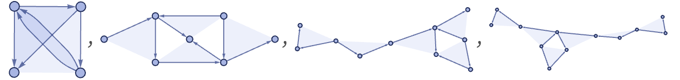
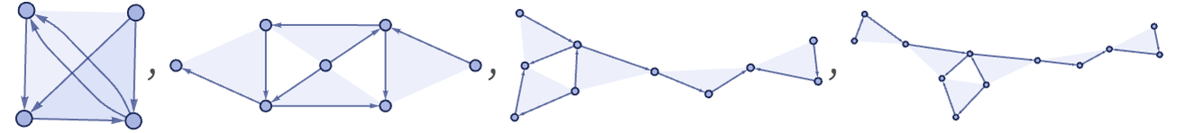
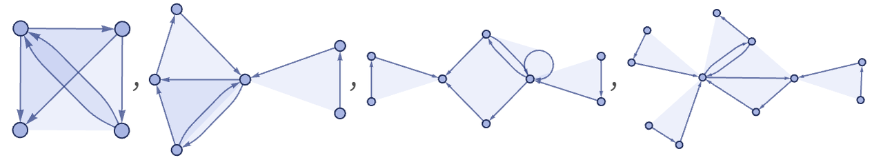
For rules with binary relations, the only symmetry operation that can operate on relations is reversal, corresponding to the permutation {2,1}. Of the 73 distinct 12 22 rules, 11 have this symmetry. Of the 4702 22 32 rules, 92 have the symmetry. Of the 40,405 22 42 rules, 363 have the symmetry. Those with the most complex behavior are:

{{1, 2}, {2, 3}} -> {{1, 2}, {1, 4}, {2, 3}, {4, 3}}
{RulePlot[ResourceFunction["WolframModel"][#1], ImageSize -> 120], ResourceFunction["WolframModel"][#1, #2, #3]["StatesPlotsList", "MaxImageSize" -> 50]} & @@ {{{1, 2}, {2, 3}} -> {{1, 2}, {1, 4}, {2, 3}, {4, 3}}, {{0, 0}, {0, 0}}, 7}
{{1, 2}, {2, 3}} -> {{1, 4}, {1, 3}, {4, 5}, {5, 3}}
{RulePlot[ResourceFunction["WolframModel"][#1], ImageSize -> 120], ResourceFunction["WolframModel"][#1, #2, #3]["StatesPlotsList", "MaxImageSize" -> 50]} & @@ {{{1, 2}, {2, 3}} -> {{1, 4}, {1, 3}, {4, 5}, {5, 3}}, {{0, 0}, {0, 0}}, 7}

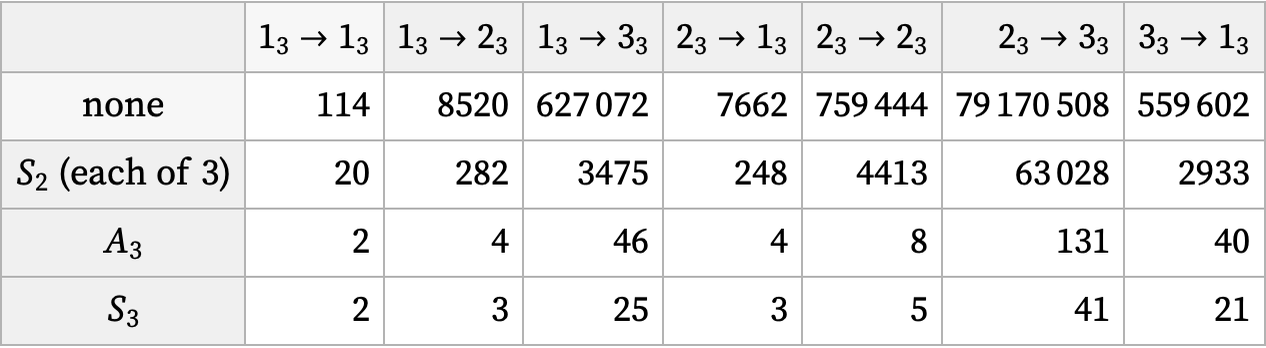
For rules with ternary relations, there are six distinct symmetry classes corresponding to the six subgroups of the symmetric group S3: no invariance, invariance under transposition of two elements (3 cases of S2) ({1,3,2}, {3,2,1} or {2,1,3} only), invariance under cyclic rotation (A3) ({2,3,1} and {3,1,2}), or invariance under any permutation (full S3). Here are the numbers of rules of various signatures with these different symmetries:

CloudGet["https://wolfr.am/LmMqWKV5"]

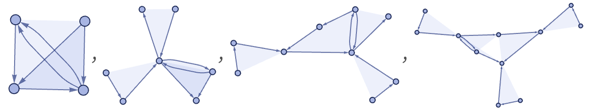
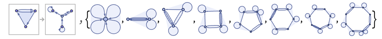
Examples of rules with full S3 symmetry include (compare 7.2):

{{1, 2, 3}, {2, 3, 1}} -> {{2, 2, 4}, {4, 3, 3}, {1, 4, 1}}
{RulePlot[ResourceFunction["WolframModel"][#1], ImageSize -> 120], ResourceFunction["WolframModel"][#1, #2, #3]["StatesPlotsList", ImageSize -> 50]} & @@ {{{1, 2, 3}, {2, 3, 1}} -> {{2, 2, 4}, {4, 3, 3}, {1, 4, 1}}, {{0, 0, 0}, {0, 0, 0}}, 7}
{{1, 2, 3}, {2, 3, 1}} -> {{4, 4, 2}, {4, 1, 4}, {3, 4, 4}}
{RulePlot[ResourceFunction["WolframModel"][#1], ImageSize -> 120], ResourceFunction["WolframModel"][#1, #2, #3]["StatesPlotsList", ImageSize -> 50]} & @@ {{{1, 2, 3}, {2, 3, 1}} -> {{4, 4, 2}, {4, 1, 4}, {3, 4, 4}}, {{0, 0, 0}, {0, 0, 0}}, 7}

An example of a rule with only cyclic (A3) symmetry is:

{{1, 2, 3}, {2, 3, 1}} -> {{1, 1, 4}, {4, 2, 2}, {3, 4, 3}}
{RulePlot[ResourceFunction["WolframModel"][#1], ImageSize -> 120], ResourceFunction["WolframModel"][#1, #2, #3]["StatesPlotsList", ImageSize -> 50]} & @@ {{{1, 2, 3}, {2, 3, 1}} -> {{1, 1, 4}, {4, 2, 2}, {3, 4, 3}}, {{0, 0, 0}, {0, 0, 0}}, 7}

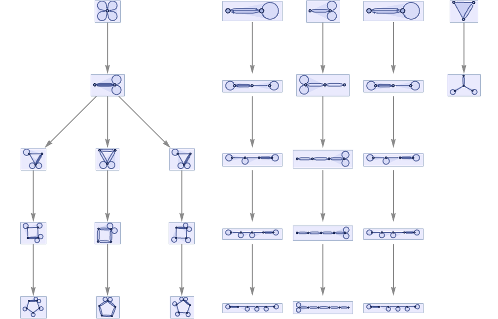
The existence of symmetry in a rule has implications for its multiway graph, effectively breaking its state transition graph into pieces corresponding to different cosets (compare [1:p963]). For example, starting from all 102 distinct 2-element ternary hypergraphs, the first completely symmetric rule above gives multiway system:

CloudGet["https://wolfr.am/LmHho8Tr"]; newgraph[ ResourceFunction["MultiwaySystem"][ "WolframModel" -> {{{1, 2, 3}, {2, 3, 1}} -> {{2, 2, 4}, {4, 3, 3}, {1, 4, 1}}}, ResourceFunction["EnumerateHypergraphs"][{{2, 3}}], 4, "StatesGraph", VertexSize -> 1], {0.9, 0.3}]

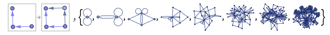
A somewhat simpler example of a completely symmetric rule is:

{{1, 2, 3}, {2, 3, 1}} -> {{1, 2, 3}, {2, 3, 1}, {3, 1, 2}}
RulePlot[ResourceFunction[ "WolframModel"][{{1, 2, 3}, {2, 3, 1}} -> {{1, 2, 3}, {2, 3, 1}, {3, 1, 2}}]]
ResourceFunction["MultiwaySystem"][ "WolframModel" -> {{{1, 2, 3}, {2, 3, 1}} -> {{1, 2, 3}, {2, 3, 1}, {3, 1, 2}}}, ResourceFunction["EnumerateHypergraphs"][{{2, 3}}], 4, "StatesGraph", VertexSize -> 1]

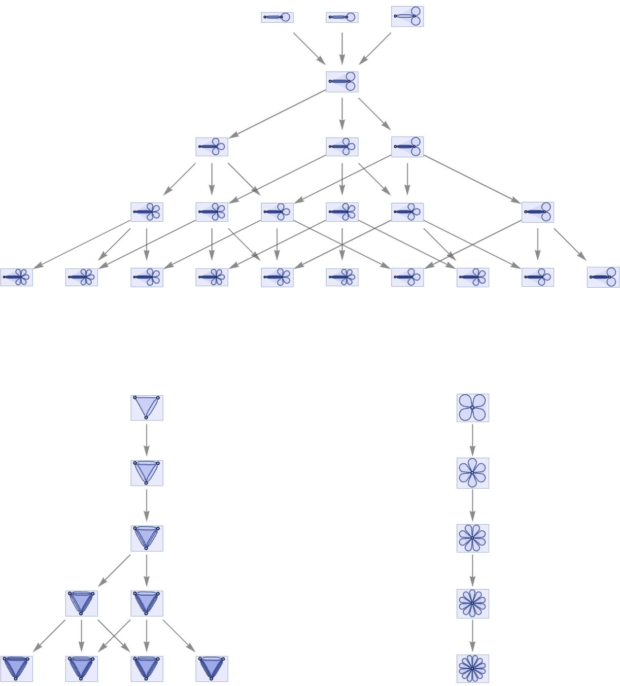
This rule has a simple conservation law: it generates new relations but not new elements. And as a result its multiway graph breaks into multiple separate components.

In general one can imagine many different kinds of conservation laws, some associated with identifiable symmetries, and some not. To get a sense of what can happen, let us consider the simpler case of string substitution systems.

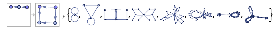
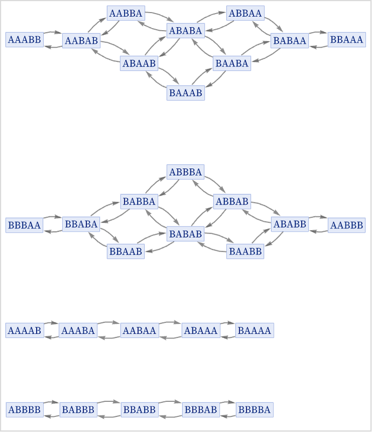
The rule (which has reversal symmetry)

{"BA" -> "AB", "AB" -> "BA"}

gives a multiway graph which consists of separate components distinguished by their total numbers of As and Bs:

Framed[ResourceFunction["MultiwaySystem"][{"BA" -> "AB", "AB" -> "BA"}, ResourceFunction["StringTuples"]["AB", 5], 8, "StatesGraph"], FrameStyle -> LightGray]

The rule

{"AA" -> "BB", "BB" -> "AA"}
Framed[ResourceFunction["MultiwaySystem"][{"AA" -> "BB", "BB" -> "AA"}, ResourceFunction["StringTuples"]["AB", 5], 8, "StatesGraph"], FrameStyle -> LightGray]

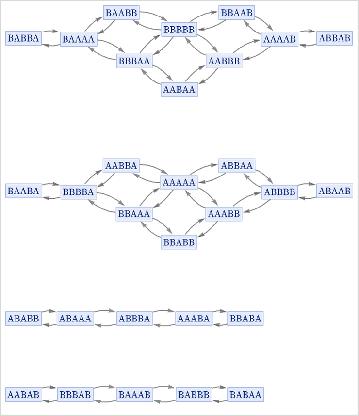
gives the same basic structure, but now what distinguishes the components is the difference in the number of ABs vs. BAs that occur in each string. In both these examples, the number of distinct components increases linearly with the length of the strings.
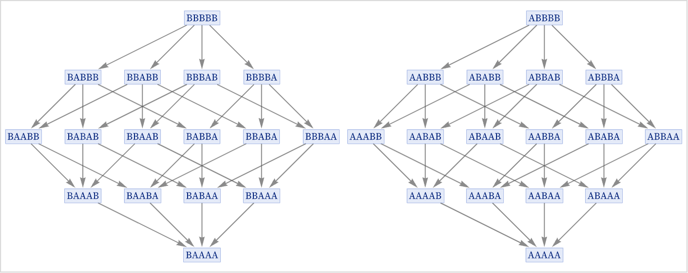
The rule

{"AA" -> "BB", "AB" -> "BA"}

already gives exactly two components, one with an even number of Bs, and one with an odd number:
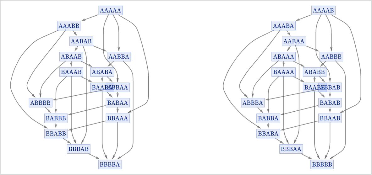
Framed[ResourceFunction["MultiwaySystem"][{"AA" -> "BB", "AB" -> "BA"}, ResourceFunction["StringTuples"]["AB", 5], 8, "StatesGraph"], FrameStyle -> LightGray]

The rule

{"AB" -> "AA", "BB" -> "BA"}

also gives two components, but now these just correspond to strings that start with A or start with B.

Framed[ResourceFunction["MultiwaySystem"][{"AB" -> "AA", "BB" -> "BA"}, ResourceFunction["StringTuples"]["AB", 5], 8, "StatesGraph", GraphLayout -> {"PackingLayout" -> "NestedGrid"}], FrameStyle -> LightGray]