6.10 Causal Disconnection

In 2.9 we discussed the fact that some rules—even though the rules themselves are connected—can lead to hypergraphs that are disconnected. And—unless one is dealing with rules with disconnected left-hand sides—any hypergraphs that are disconnected must also be causally disconnected.

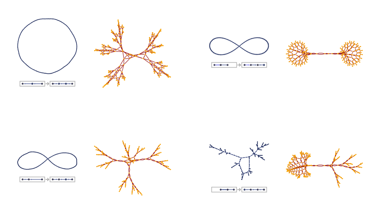
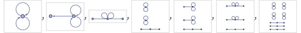
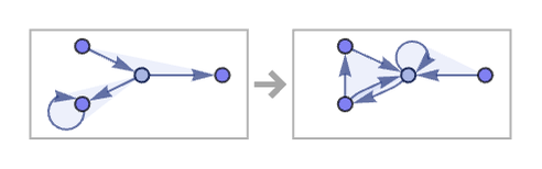
As a simple example of what can happen, consider the rule:

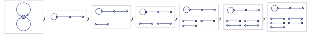
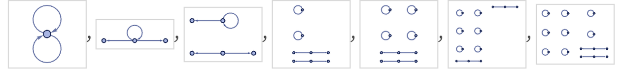
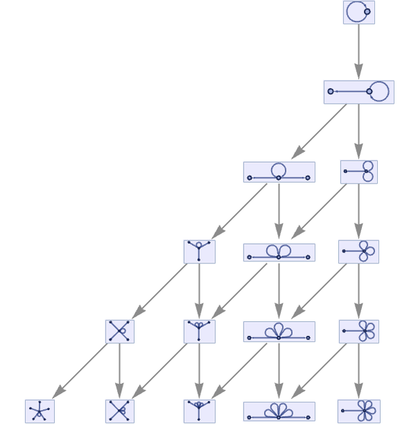
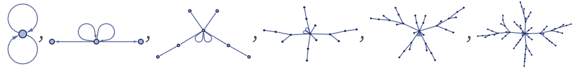
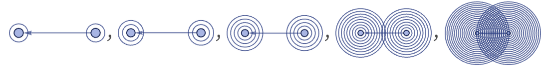
The evolution of this rule quickly leads to disconnected hypergraphs:

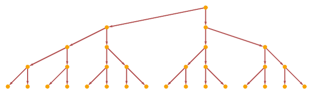
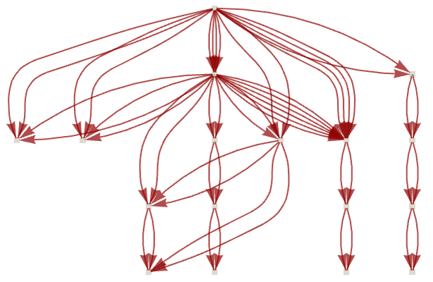
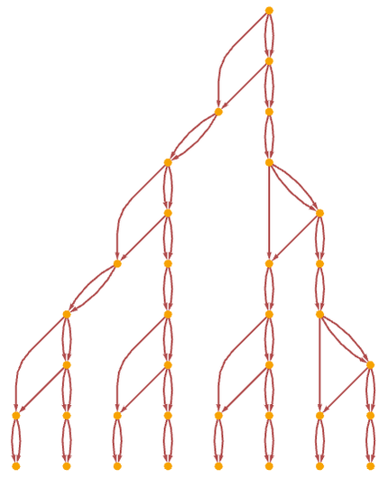
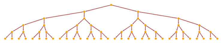
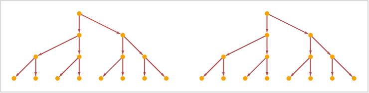
The corresponding causal graph is a tree:

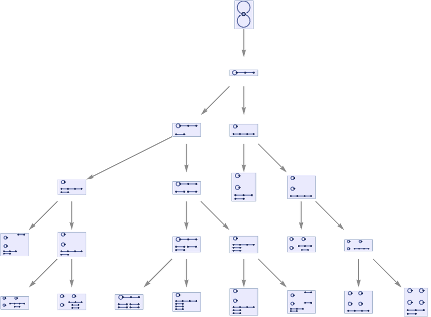
In this particular case, the different branches happen to correspond to isomorphic hypergraphs, so that in our usual way of creating a multiway graph, this rule leads to a connected multiway graph, which even shows causal invariance:

(Note that causal invariance is in a sense easier to achieve with disconnected hypergraphs, because there is no possibility of overlap, or of ambiguity in updates.)

In the case of an extremely simple rule like

the evolution is immediately disconnected

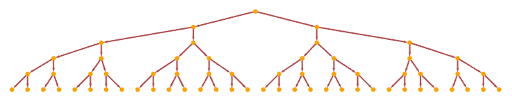
the causal graph is a tree

but the multiway graph consists of a simple “counting” sequence of states:

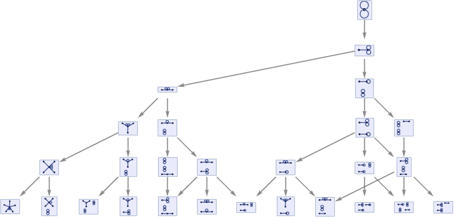
In other rules, the disconnected pieces are not isomorphic, and the multiway graph can split. An example where this occurs is the rule:

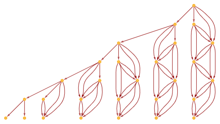
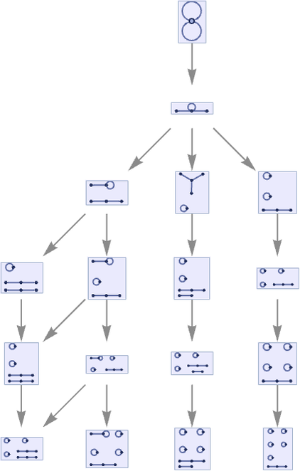
The multiway graph in this case is a tree:

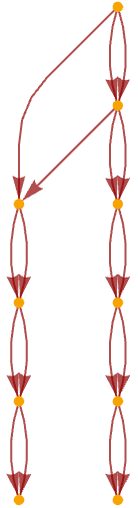
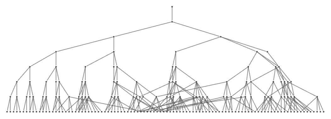
The multiway causal graph, however, does not have an exponential tree structure, but instead effectively just has one branch for each disconnected component in the hypergraph:

As a result, for this rule the ordinary causal graph has a simple, sequential form:

As a related example, consider the rule:

In this case, the multiway graph has the two-branch form

and the multiway causal graph has the similarly two-branch form

though the ordinary causal graph is still just:

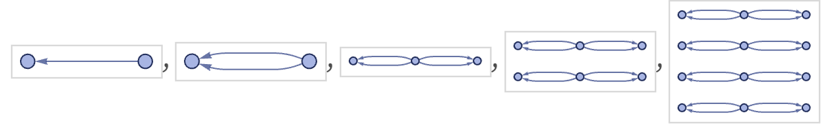
Sometimes there can be multiple branches in both the multiway graph and the ordinary causal graph. An example occurs in the rule

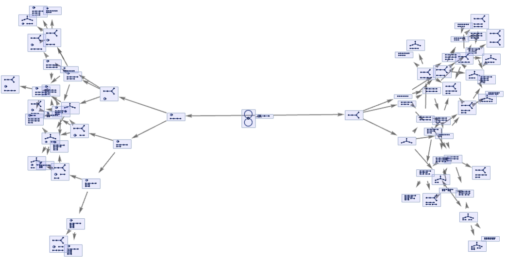
where the multiway graph is

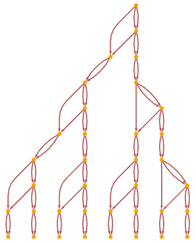
the multiway causal graph is

and the ordinary causal graph is:

Is it possible to have both an infinitely branching multiway graph, and an infinitely branching ordinary causal graph? One of the issues is that in general it can be undecidable whether this is ultimately infinite branching. Consider for example the rule:

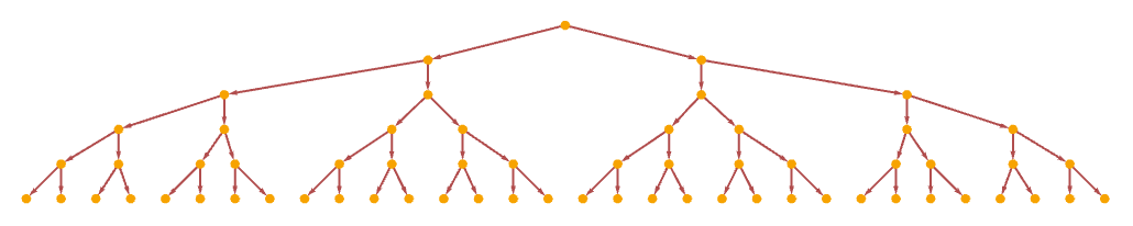
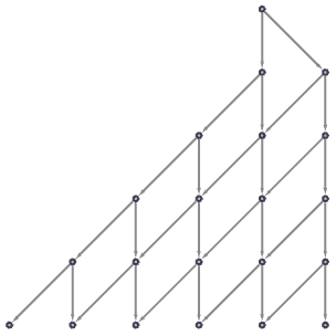
The ordinary causal graph for this rule has the form

or in a different rendering after more steps:

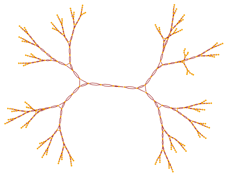
The multiway causal graph in this case is:

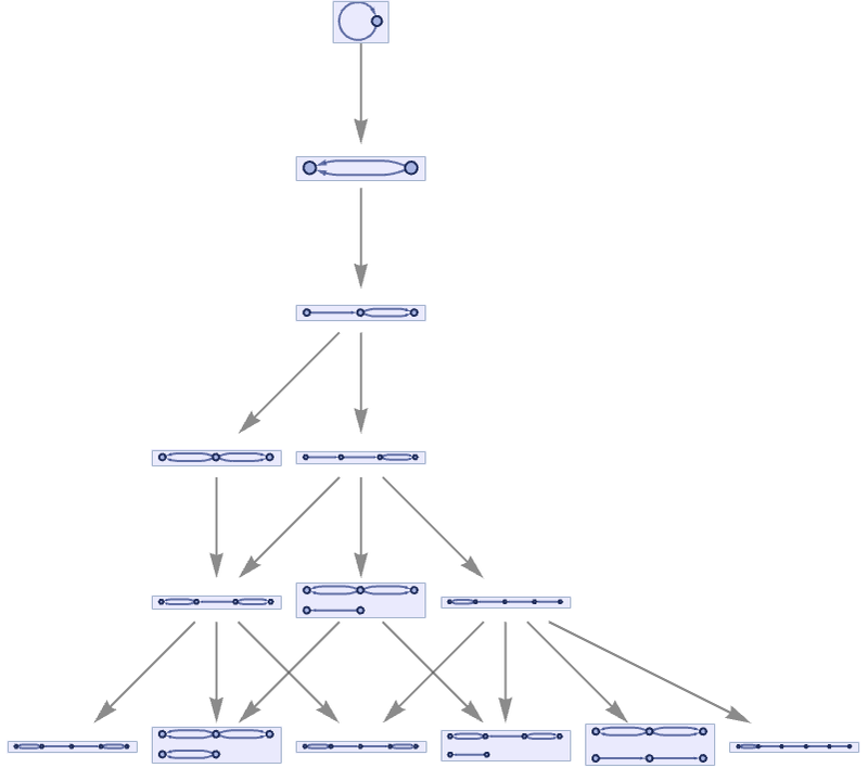
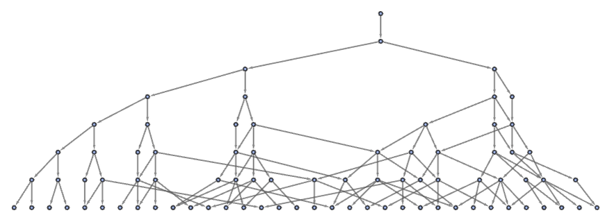
But now the multiway graph is:

Continuing for more steps yields:

But while it is fairly clear that this multiway graph does not show causal invariance, it is not clear whether it will branch forever or not.

As a similar example, consider the rule:

This yields the same ordinary causal graph as the previous rule

but now its multiway graph has a form that appears slightly more likely to branch forever:

All the examples we have seen so far involve explicit disconnection of hypergraphs. However, it is also possible to have causal disconnection even without explicit disconnection of hypergraphs. As a very simple example, consider the rule:

The causal graph in this case is

although the multiway graph is just:

For the rule

the causal graph is again a tree

but now the multiway graph is:

The rule

gives exactly the same causal graph, but now its hypergraph is a tree:

Like some of the rules shown above, its multiway graph is somewhat complex:

It is actually fairly common to have causal graphs that look like the corresponding hypergraphs in the case of rules where effectively only one update happens at a time. An example occurs in the case of the rule (see 3.10):

So far, we have only considered fairly minimal initial conditions. But as soon as it is possible to have multiple independent events occur in the initial conditions, it is also possible to get completely disconnected causal graphs. (Note that if an “initial creation event” to create the initial conditions was added, then the causal graphs would again be connected.) As an example of disconnected causal graphs, consider the rule

with an initial condition consisting of connected unary relations:

This rule yields a disconnected causal graph:

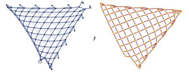
The multiway graph in this case is connected, and shows causal invariance:

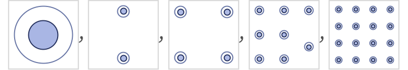
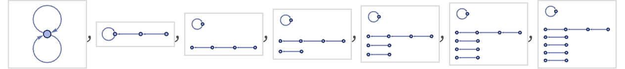
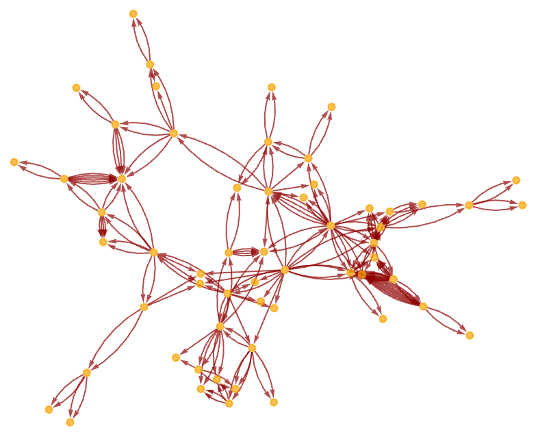
Sometimes the relationship between disconnection in the hypergraph and the existence of disconnected causal graphs can be somewhat complex. This shows results for the rule above with initial conditions consisting of increasing numbers of self-loops:

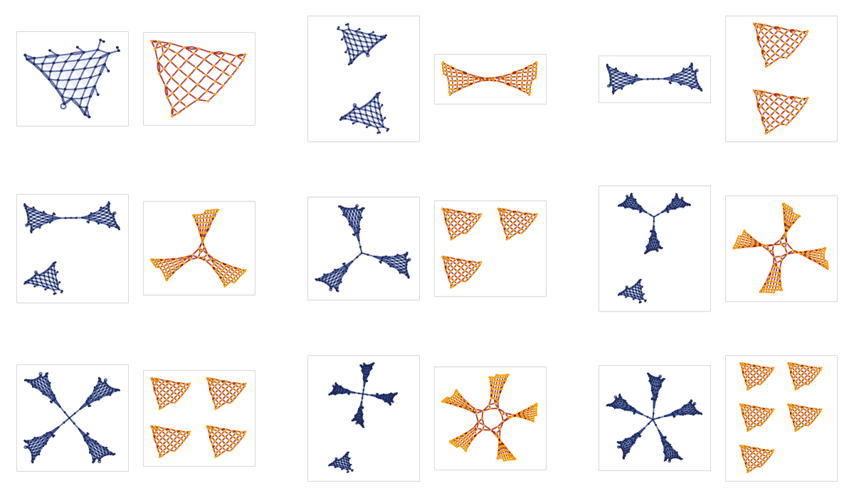
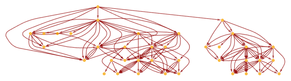
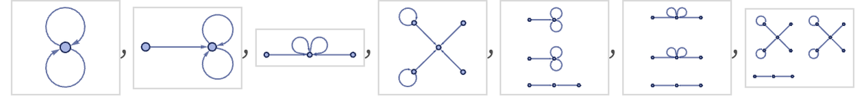
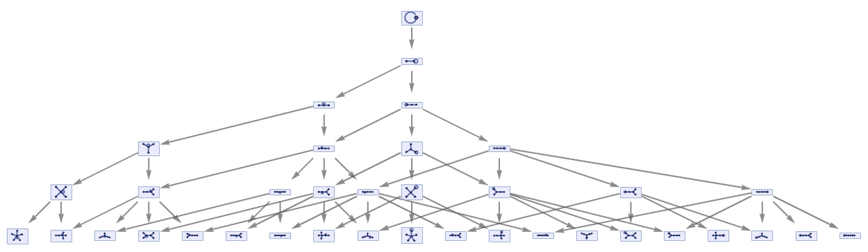
Even with rather simple rules, the forms of branching in causal graphs can be quite complex—even when the actual hypergraphs remain simple. Here are a few examples: