A Class of Models with the Potential to Represent Fundamental Physics
  1. Introduction
  2. Basic Form of Models
  3. Typical Behaviors
  4. Limiting Behavior and Emergent Geometry
  5. The Updating Process for String Substitution Systems
  6. The Updating Process in Our Models
  7. Equivalence and Computation in Our Models
  8. Potential Relation to Physics
  9. Additional Material
  10. References
  11. Index

6.4 Testing for Causal Invariance

Testing for causal invariance in our models is similar in principle to the case of strings. Failure of causal invariance is again the result of branch pairs that do not resolve. And just like for strings, it is possible to test for total causal invariance by determining whether a certain finite set of core branch pairs resolve. (Again in analogy with strings, the finiteness of this set is a consequence of the finiteness of the hypergraphs involved in our rules.)

The core branch pairs that we need to test represent the minimal cases of overlap between left-hand sides of rulesor, in a sense, the minimal unifications of the hypergraphs that appear. For the two hypergraphs

{ResourceFunction["WolframModelPlot"][{{a, b}, {a, a}}, VertexLabels -> Automatic, EdgeStyle -> Blue], ResourceFunction["WolframModelPlot"][{{x, y}, {x, z, w}}, VertexLabels -> Automatic, EdgeStyle -> Red]}

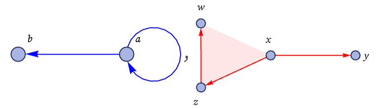
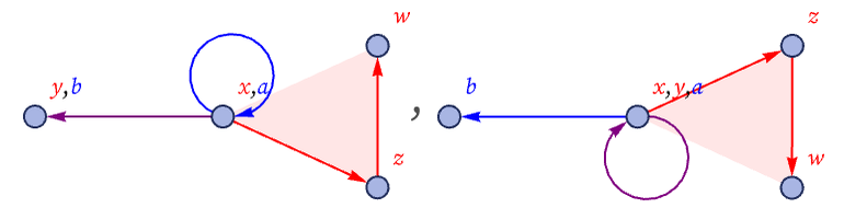
there are two possible unifications (where the purple edge shows the overlap):

CloudGet["https://wolfr.am/LlJ5vv0j"];\ WMUnificationsPlot[{{x, y}, {x, z, w}}, {{a, b}, {a, a}}, VertexLabels -> Automatic]

For a single rule with left-hand side

{{x, y}, {x, z}}

the core branch pairs arise from unifications associated with the possible self-overlaps of this small hypergraph. Representing two copies of the hypergraph as

{ResourceFunction["WolframModelPlot"][{{x, y}, {x, z}}, VertexLabels -> Automatic, EdgeStyle -> Blue], ResourceFunction["WolframModelPlot"][{{a, b}, {a, c}}, VertexLabels -> Automatic, EdgeStyle -> Red]}

the possible unifications are:

CloudGet["https://wolfr.am/LlJ5vv0j"];\ WMUnificationsPlot[{{a, b}, {a, c}}, {{x, y}, {x, z}}, ImageSize -> 120, VertexLabels -> Automatic]

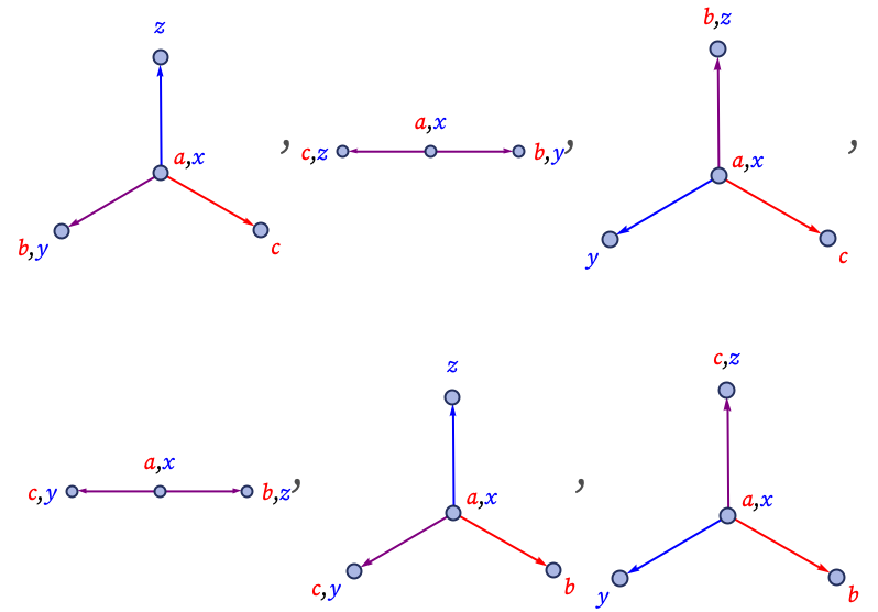
In the case of strings, all that matters is what symbols appear within the unification. In the case of hypergraphs, one also has to know how the unification in effect “attaches”, and so one has to distinguish different labelings of the nodes.

Starting from the unifications, one applies the rule to find what branch pairs can be produced. These branch pairs form the core set of branch pairs for the ruleand determining whether the rule is causal invariant then becomes a matter of finding out whether these branch pairs resolve.

In the case of

{{x, y}, {x, z}} -> {{x, y}, {x, w}, {y, w}, {z, w}}

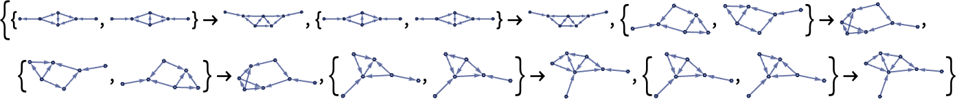
the application of the rule to the unifications above yields the following 58 core branch pairs:

Map[ResourceFunction["WolframModelPlot"][#, ImageSize -> 30] &, ResourceFunction["CanonicalBranchPairs"][ "WolframModel" -> {{{x, y}, {x, z}} -> {{x, z}, {x, w}, {y, w}, {z, w}}}, 0, "IncludeSelfPairs" -> False]["Unresolved"], {2}]

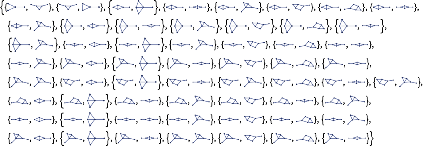
Running the rule for one step yields resolutions for 6 of these branch pairs:

With[{f = ResourceFunction["WolframModelPlot"][#, ImageSize -> 60, "ArrowheadLength" -> 0.3] &}, Map[(f /@ First[#]) -> (f@ Last[#]) &, {{{{1, 2}, {1, 3}, {1, 5}, {2, 3}, {2, 4}, {4, 3}, {6, 4}}, {{1, 2}, {1, 3}, {1, 4}, {2, 3}, {2, 4}, {5, 3}, {6, 4}}} -> {{1, 2}, {1, 3}, {1, 4}, {2, 3}, {2, 4}, {2, 5}, {5, 3}, {6, 4}, {7, 5}}, {{{1, 2}, {1, 3}, {1, 4}, {2, 3}, {2, 4}, {5, 3}, {6, 4}}, {{1, 2}, {1, 3}, {1, 5}, {2, 3}, {2, 4}, {4, 3}, {6, 4}}} -> {{1, 2}, {1, 3}, {1, 4}, {2, 3}, {2, 4}, {2, 5}, {5, 3}, {6, 4}, {7, 5}}, {{{1, 2}, {1, 3}, {1, 4}, {2, 3}, {5, 3}, {5, 4}, {6, 4}}, {{1, 2}, {1, 3}, {1, 4}, {2, 3}, {4, 5}, {5, 3}, {6, 5}}} -> {{1, 2}, {1, 3}, {1, 4}, {2, 3}, {2, 4}, {5, 3}, {5, 6}, {6, 4}, {7, 6}}, {{{1, 2}, {1, 3}, {1, 4}, {2, 3}, {4, 5}, {5, 3}, {6, 5}}, {{1, 2}, {1, 3}, {1, 4}, {2, 3}, {5, 3}, {5, 4}, {6, 4}}} -> {{1, 2}, {1, 3}, {1, 4}, {2, 3}, {2, 4}, {5, 3}, {5, 6}, {6, 4}, {7, 6}}, {{{1, 2}, {1, 3}, {1, 5}, {2, 3}, {4, 2}, {4, 3}, {6, 2}}, {{1, 2}, {1, 3}, {1, 4}, {2, 3}, {3, 4}, {5, 3}, {6, 4}}} -> {{1, 2}, {1, 3}, {1, 4}, {2, 3}, {2, 4}, {5, 2}, {5, 3}, {6, 2}, {7, 4}}, {{{1, 2}, {1, 3}, {1, 4}, {2, 3}, {3, 4}, {5, 3}, {6, 4}}, {{1, 2}, {1, 3}, {1, 5}, {2, 3}, {4, 2}, {4, 3}, {6, 2}}} -> {{1, 2}, {1, 3}, {1, 4}, {2, 3}, {2, 4}, {5, 2}, {5, 3}, {6, 2}, {7, 4}}}]]

Running for another step resolves no additional branch pairs.

Will the rule turn out to be causal invariant in the end? As a comparison, consider the rule

{{x, y}, {x, z}} -> {{y, w}, {y, z}, {w, x}}

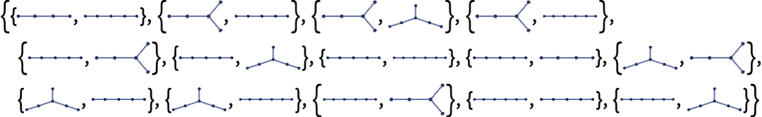
discussed in the previous subsection. This rule starts with 14 core branch pairs:

Monitor[Do[ tcrits[i] = ResourceFunction["CanonicalBranchPairs"][ "WolframModel" -> {{{1, 2}, {1, 3}} -> {{2, 4}, {2, 3}, {4, 1}}}, i, "IncludeSelfPairs" -> False];, {i, 0, 3}], i]; Map[ResourceFunction["WolframModelPlot"][#, ImageSize -> 40] &, tcrits[0]["Unresolved"], {2}]

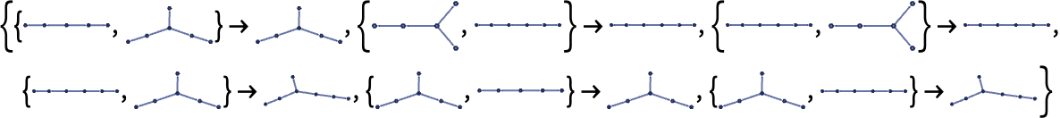
After one step, 6 of them resolve:

Monitor[Do[ tcrits[i] = ResourceFunction["CanonicalBranchPairs"][ "WolframModel" -> {{{1, 2}, {1, 3}} -> {{2, 4}, {2, 3}, {4, 1}}}, i, "IncludeSelfPairs" -> False, "GiveResolvents" -> True];, {i, 0, 3}], i]; With[{f = ResourceFunction["WolframModelPlot"][#, ImageSize -> 50] &}, Map[(f /@ First[#]) -> (f@Last[#]) &, tcrits[1]["Resolved"]]]

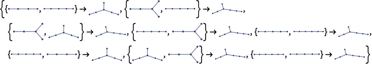
Then after another step the 8 remaining ones resolve, establishing that the rule is indeed causal invariant:

Monitor[Do[ tcrits[i] = ResourceFunction["CanonicalBranchPairs"][ "WolframModel" -> {{{1, 2}, {1, 3}} -> {{2, 4}, {2, 3}, {4, 1}}}, i, "IncludeSelfPairs" -> False, "GiveResolvents" -> True];, {i, 0, 3}], i]; With[{f = ResourceFunction["WolframModelPlot"][#, ImageSize -> 50] &}, Map[(f /@ First[#]) -> (f@Last[#]) &, Complement[tcrits[2]["Resolved"], tcrits[1]["Resolved"]]]]

But in general there is no upper bound on the number of steps it can take for core branch pairs to resolve. Perhaps the fact that so many additional branch pairs are generated at each step in the rule {{x,y},{x,z}}{{x,z},{x,w},{y,w},{z,w}} makes it seem unlikely that they will all resolve, but ultimately this is not clear.

And even if the rule does not show total causal invariance, it is still perfectly possible that it will be causal invariant for the particular set of states generated from a certain initial condition. However, determining this kind of partial causal invariance seems even more difficult than determining total causal invariance.

Note that if one looks at all 4702 22 32 rules, the largest number of core branch pairs for any rule is 554; the largest number that resolve in 1 step is 132, and the largest number that remain unresolved is 430.