 download pdf
  ARXIV
ARXIV peer review
Even if we do not know that a rule is causal invariant, we can still construct a causal graph for it based on a particular updating order—and often different updating orders will give at least similar causal graphs.
Thus, for example, for the rule
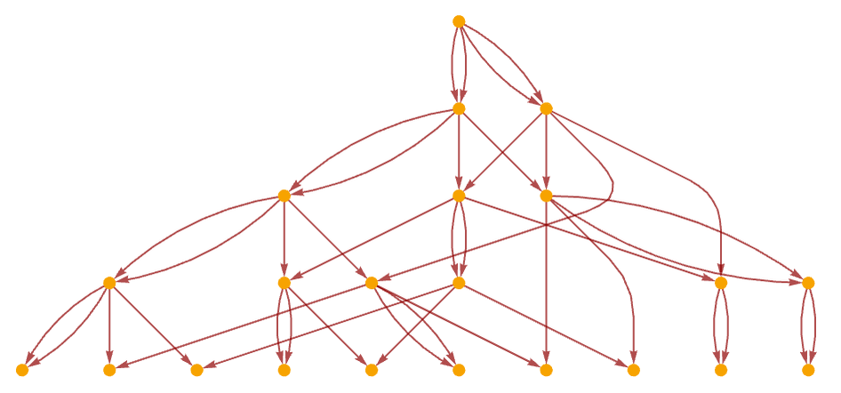
applying our standard updating order for 5 steps gives the causal graph:
Continuing for 10 steps, we get:
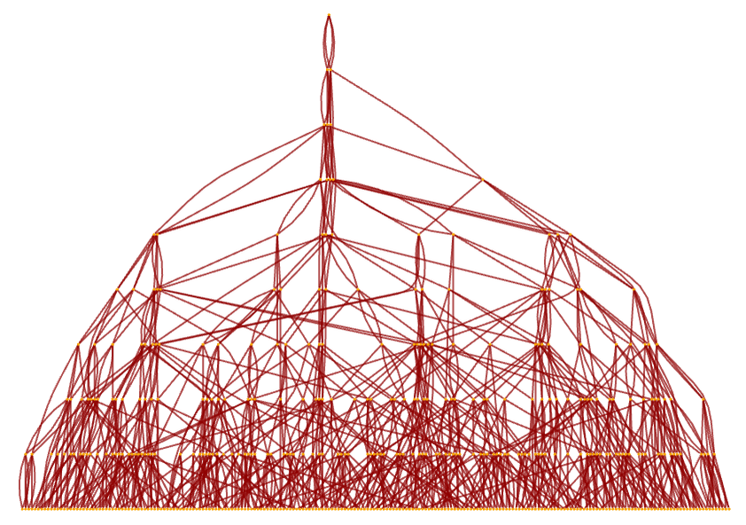
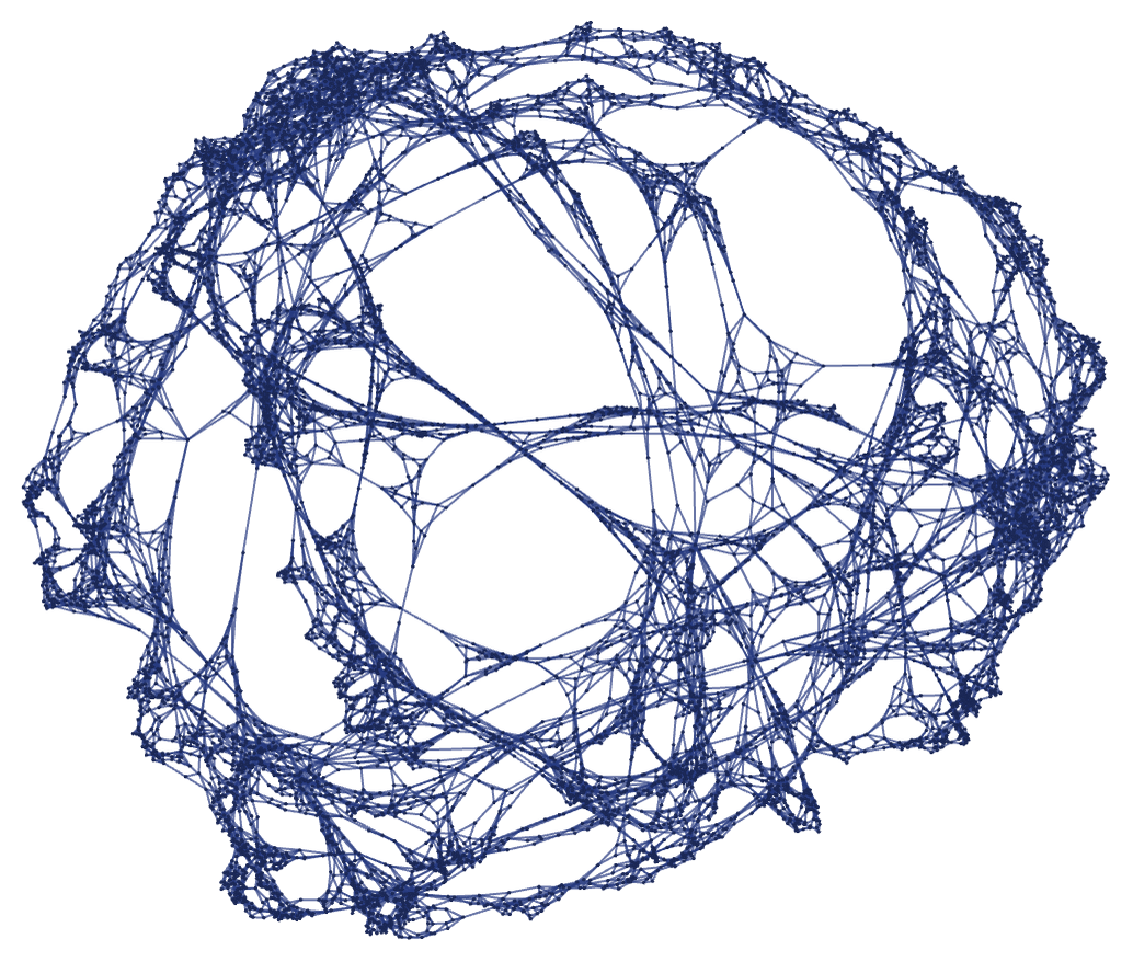
This can also be rendered as:
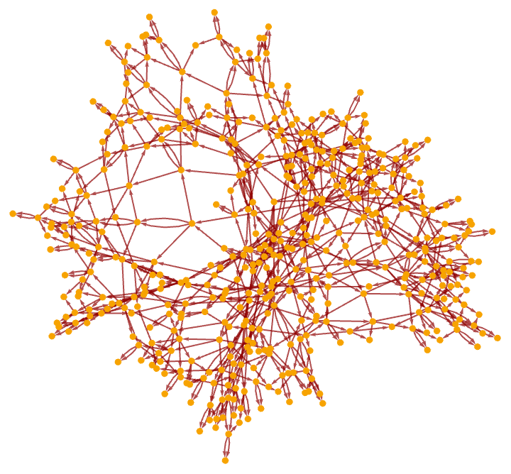
After 15 steps, there are 10,346 nodes:
In effect the successive steps in the evolution of the system correspond to successive slices through this causal graph. In the case of causal invariant rules, any possible updating order must correspond to a possible causal foliation of the graph. But here we can at least say that the foliation obtained by looking at successive layers starting from the root corresponds to successive steps of evolution with our standard updating order.
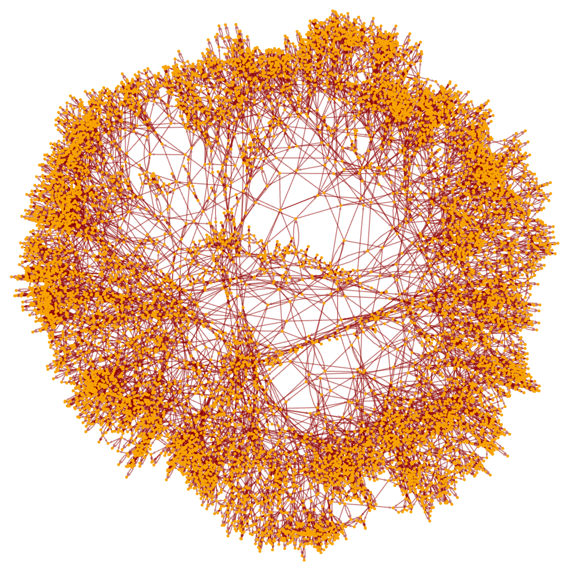
For any system whose evolution continues infinitely, the causal graph will ultimately be infinite. But by slicing the graph as we have above, we are effectively showing the events that contribute to forming the state of the system after 15 steps of evolution (in this case, with our standard updating order):
(Note that with this particular rule, the vast majority of relations that appear at step 15 were added specifically at that step, so in a sense most of the state at step 15 is associated just with the slice of the causal graph at layer 15.)