6.7 Typical Causal Graphs

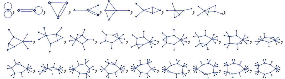
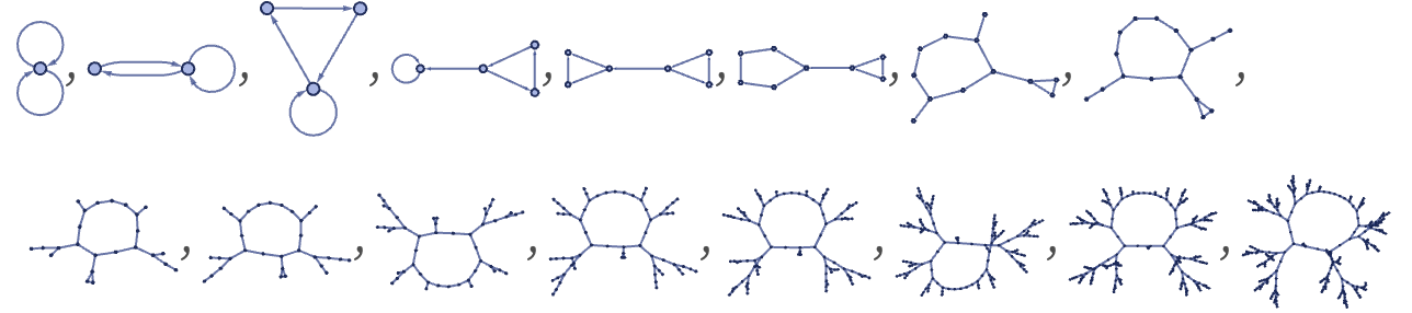
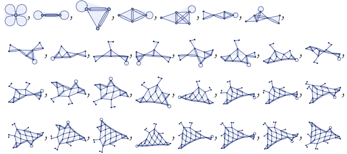
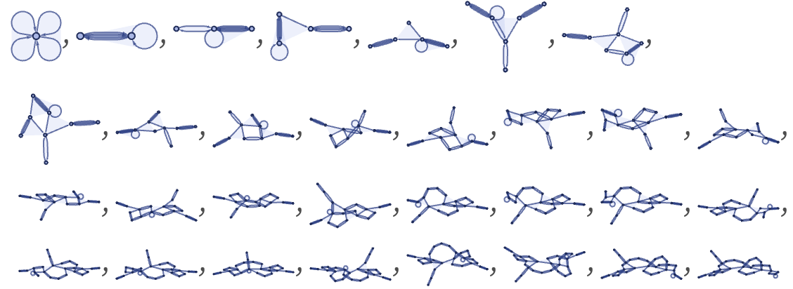
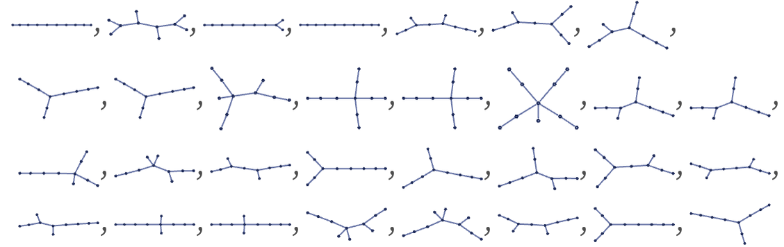
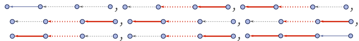
As we discussed in 5.12, causal graphs for string substitution systems tend to have fairly simple structures. Causal graphs for our models tend to be considerably more complicated, and even among 2₂  3₂ rules considerable diversity is observed. A typical random sample of different forms is:

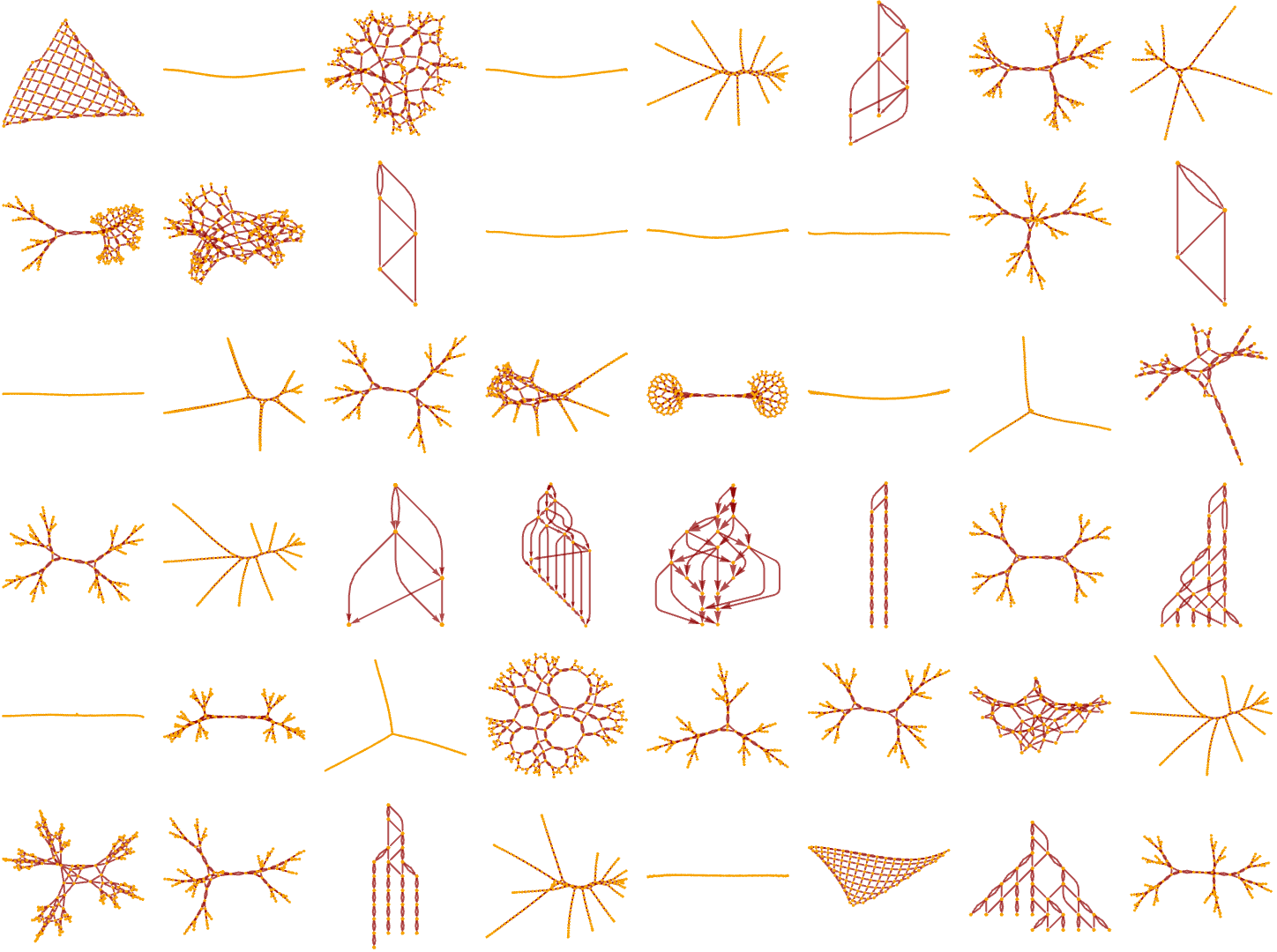
Even rules whose states seem quite simple can produce quite complex causal graphs:

As a first example, consider the rule:

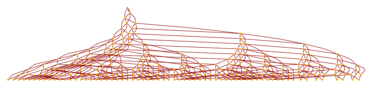
At each step, the self-loop just adds a relation, and effectively moves around the growing loop:

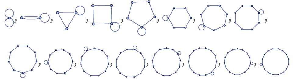
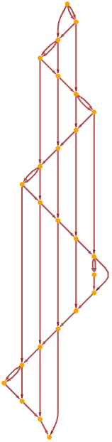
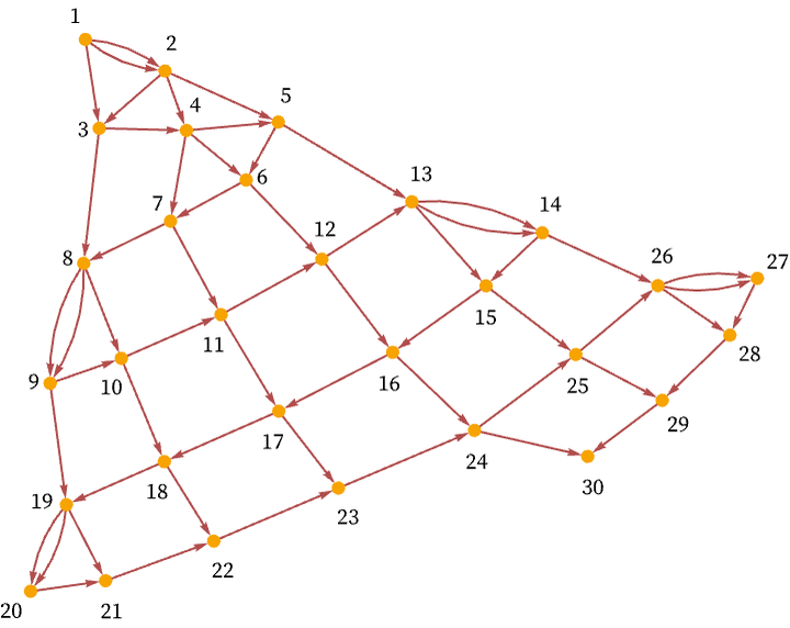
The causal graph captures the causal connections created by the self-loop encountering the same relations again after it goes all the way around:

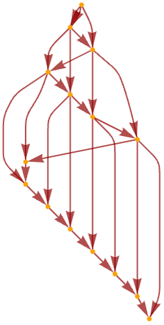
The structure gets progressively more complicated:

Re-rendering this gives

or after 500 steps:

As another example, consider the rule:

Here are the first 25 steps in its evolution (using our standard updating order):

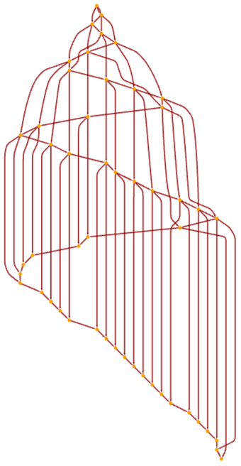
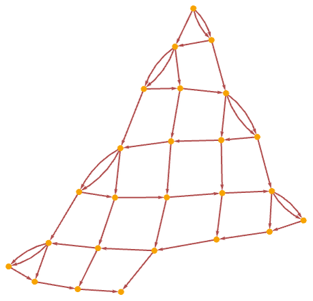
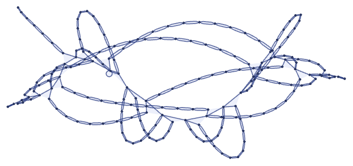
After a few steps all that happens is that there is a small structure that successively moves around the loop creating new “hairs”. The causal graph (here shown after 25 steps) captures this process:

An alternative rendering shows that a grid structure emerges:

Here are the corresponding results after 100 steps:

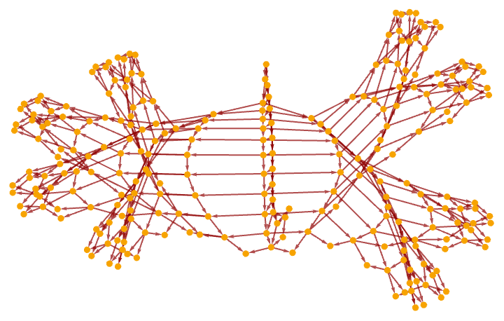
As a somewhat different example, consider the rule:

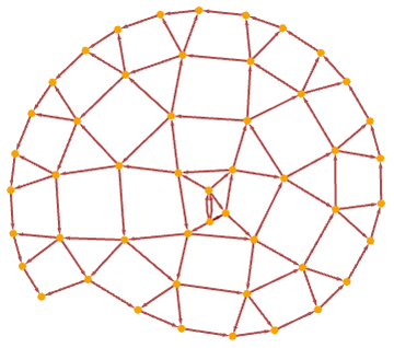
After the same number of steps, one can effectively see the separate trees in the causal graph:

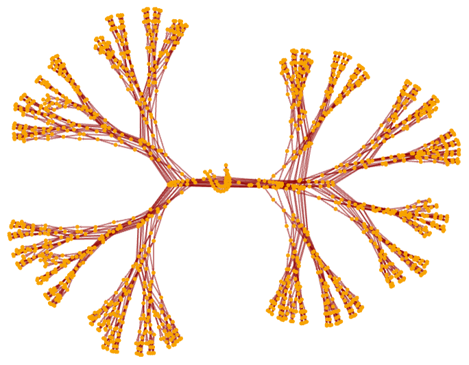
Re-rendering the causal graph, it has a structure that is quite similar to the actual state of the system:

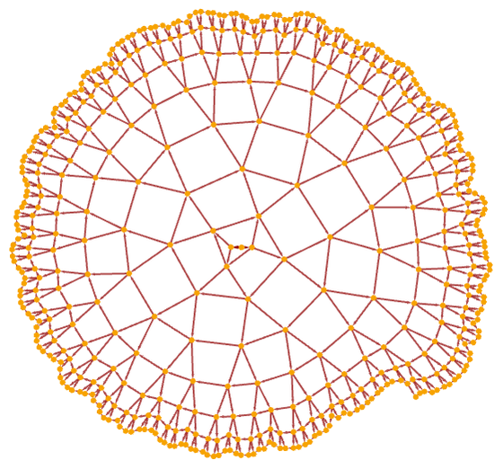
Continuing for a few more steps, a definite tree structure emerges:

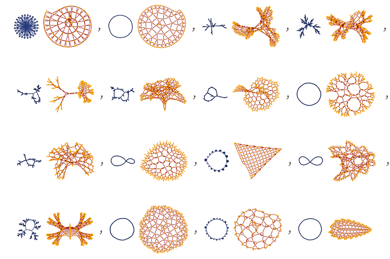
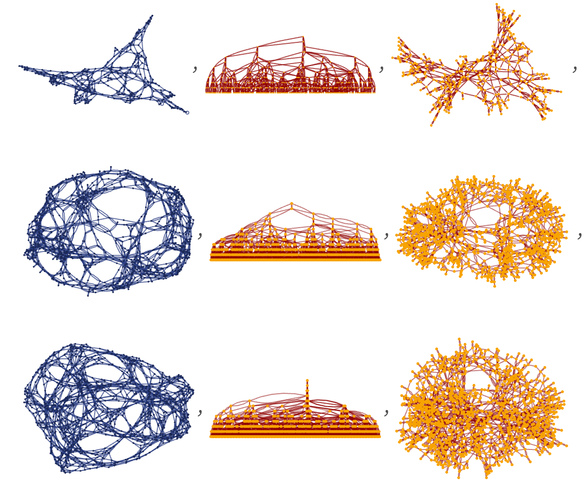
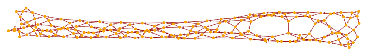
It is not uncommon for a causal graph to “look like” the actual hypergraph generated by one of our models. For example, rules that produce globular structures tend to produce similar “globular” causal graphs (here shown for three 2₂  4₂ rules from section 3):

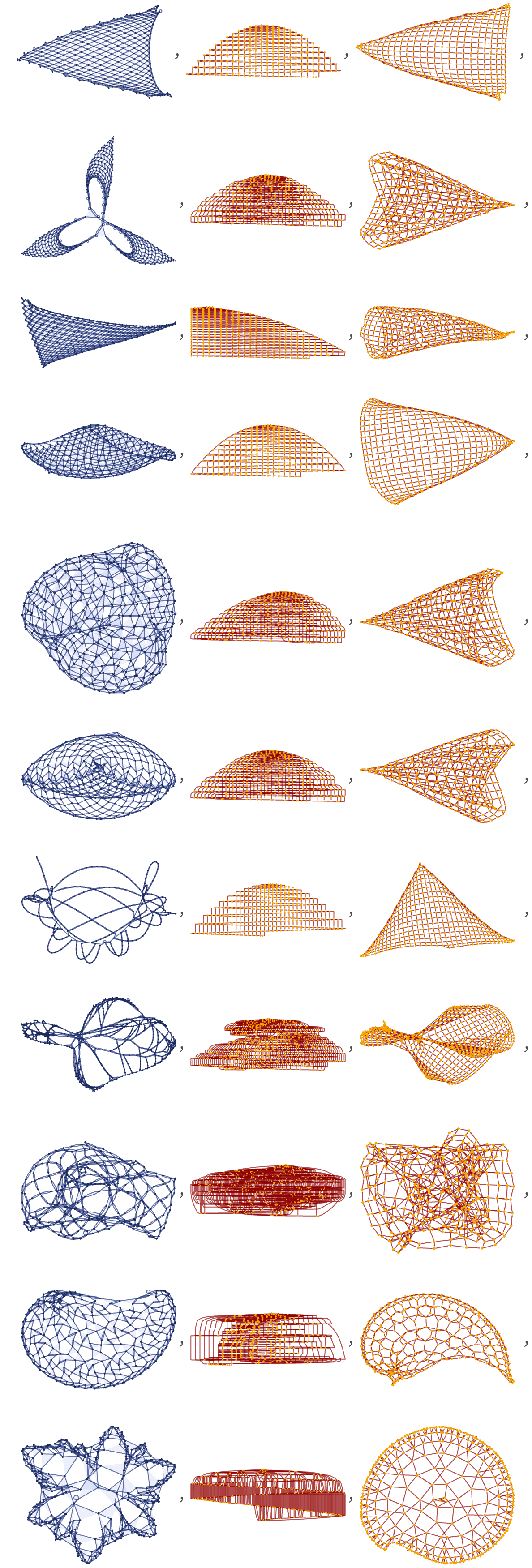
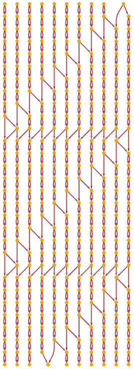
Rules that exhibit slow growth often yield either grid-like or “hyperbolic” causal graphs (here shown for some 2₃  3₃ rules from section 3):

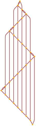
A typical source of grid-like causal graphs [1:p489] is rules where in a sense only one thing ever happens at a time, or, in effect, the rules operate like a mobile automaton [1:3.3] or a Turing machine, with a single active element. As an example, consider the rule (see 3.10):

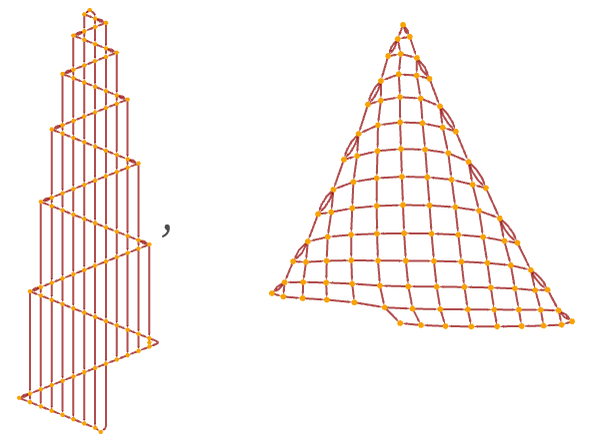
Updates can only occur at the position of the self-loop, which progressively “moves around”, “knitting” a grid pattern. The causal graph captures the fact that “only one thing happens at a time”:

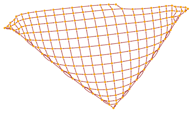
But what is notable is that if we ask about the overall causal relationships between events, we realize that even events that happened many steps apart in the evolution as shown here are actually directly causally connected, because in a sense “nothing else happened in between”. Re-rendering the causal graph illustrates this, and shows how a grid is built up:

Sometimes the actual growth process can be more complicated, as in the case of the rule

After 200 steps this yields:

And after 1000 steps it gives:

But despite this elaborate structure, the causal graph is very simple:

After 200 steps, the grid structure is clear:

Sometimes the causal graph can locally be like a grid, while having a more complicated overall topological structure. Consider for example the rule:

After 200 steps this gives:

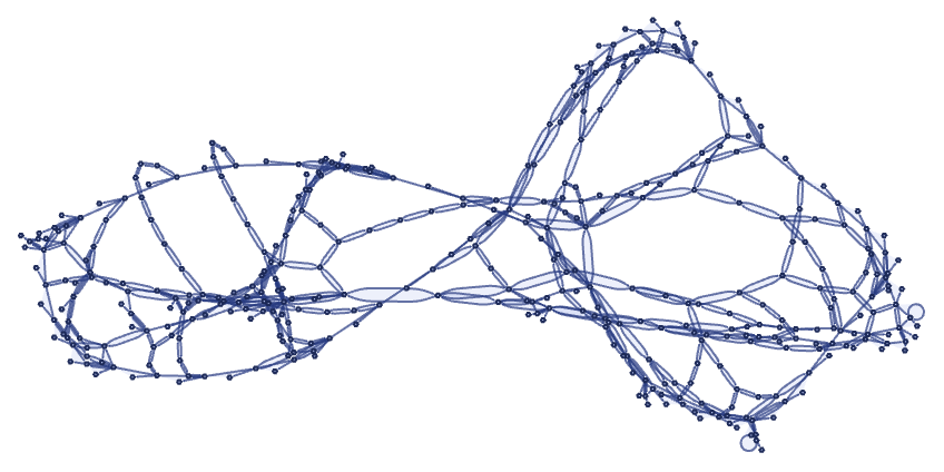
The corresponding causal graph is:

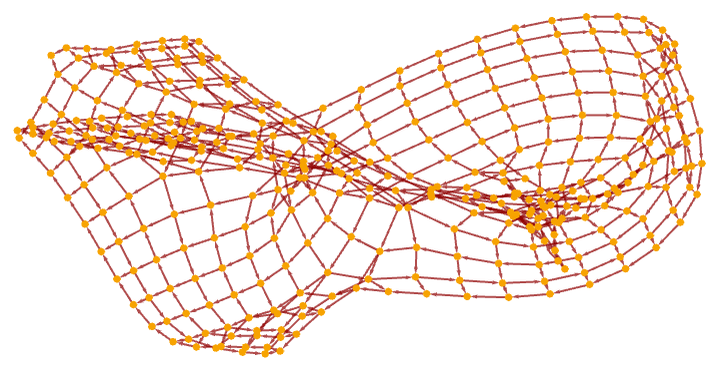
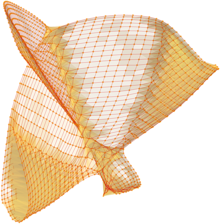
After 1000 steps with surface reconstruction this gives:

Rules (such as those with signature 2₂  2₂) that cannot exhibit growth inevitably terminate or repeat, thus leading to causal graphs that are either finite or repetitive—but may still have fairly complex structure. Consider for example the rule (compare 3.15):

Evolution from a chain of 9 relations leads to a 31-step transient, then a 9-step cycle:

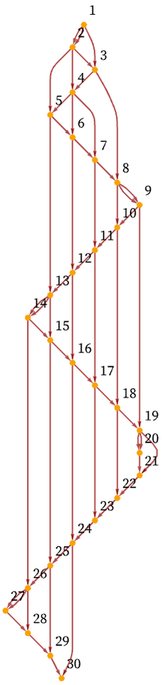
The first 30 layers in the causal graph are:

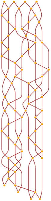
In an alternative rendering, the graph is:

After 50 more steps, the repetitive structure becomes clear:

Sometimes the structure of the causal graph may be very much a reflection of the updating order used. Consider for example the rather trivial “identity” rule:

Starting with a chain of 3 relations, this shows update events according to our standard updating order (note that the same relation can be both created and destroyed at a particular step):

The corresponding causal graph is:

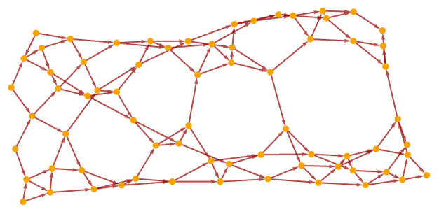
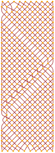
For a chain of length of 21 the causal graph consists largely of independent regions—except for the connection created by updates fitting differently at different steps:

Re-rendering this gives a seemingly elaborate structure:

After 100 steps, though, its repetitive character becomes clear:

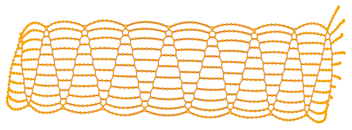
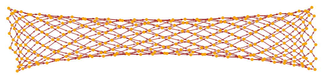
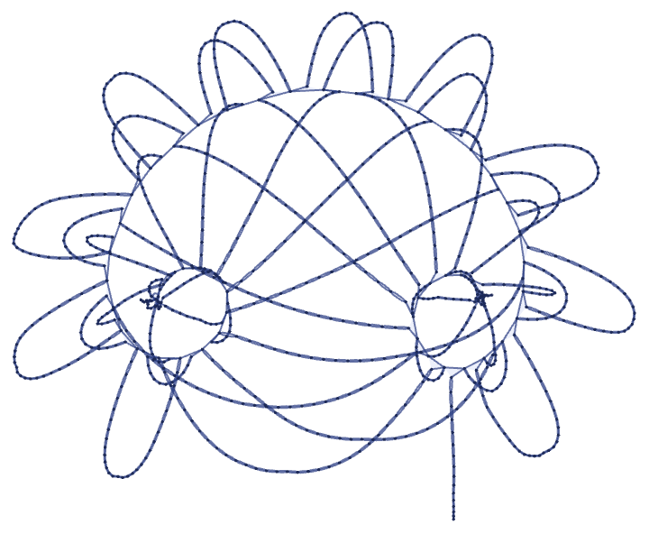
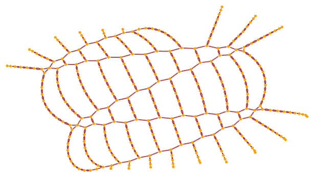
Note that if the initial condition is a ring rather than a chain, one gets

together with the tube-like structure: