3.4 Rules Depending on a Single Unary Relation

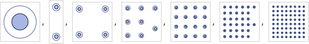
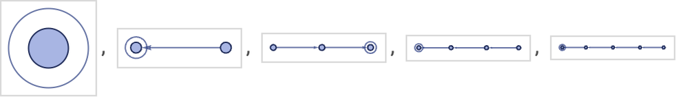
The very simplest possible rules are ones that transform a single unary relation, for example the 1₁  2₁ rule:

{{x}} -> {{x}, {y}}

RulePlot[ResourceFunction["WolframModel"][{{x}} -> {{x}, {y}}], "RulePartsAspectRatio" -> 1.99]

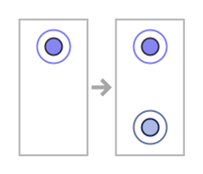
This rule generates a disconnected hypergraph, containing 2ⁿ disconnected unary hyperedges at step n:

Framed[#, ImageSize -> Tiny, FrameStyle -> LightGray] & /@ ResourceFunction["WolframModel"][{{x}} -> {{x}, {y}}, {{1}}, 6, "StatesPlotsList"]

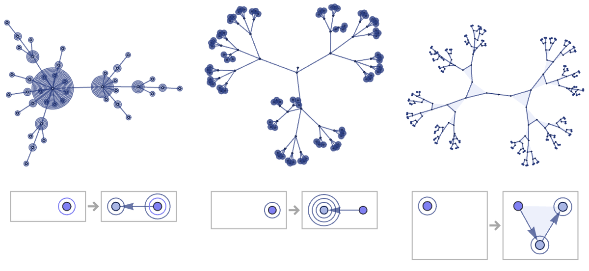
To get less trivial behavior, one must introduce at least one binary relation. With the 1₁  1₂1₁ rule

{{x}} -> {{x, y}, {x}}

RulePlot[ResourceFunction["WolframModel"][{{x}} -> {{x, y}, {x}}]]

one just gets a figure with progressively more binary-edge “arms” being added to the central unary hyperedge:

Framed[#, ImageSize -> Tiny, FrameStyle -> LightGray] & /@ ResourceFunction["WolframModel"][{{x}} -> {{x, y}, {x}}, {{1}}, 6, "StatesPlotsList"]

The rule

{{x}} -> {{x, y}, {y}}

RulePlot[ResourceFunction["WolframModel"][{{x}} -> {{x, y}, {y}}]]

produces a growing linear structure, progressively “extruding” binary edges from the unary hyperedge:

Framed[#, ImageSize -> Small, FrameStyle -> LightGray] & /@ ResourceFunction["WolframModel"][{{x}} -> {{x, y}, {y}}, {{1}}, 4, "StatesPlotsList"]

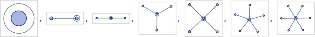
With two unary relations and one binary relation (signature 1₁  1₂2₁) there are 16 possible rules; after 4 steps starting from a single unary relation, these give:

GraphicsGrid[ Partition[ Labeled[ Framed[ ResourceFunction["WolframModelPlot"][ ResourceFunction["WolframModel"][#, {{1}}, 4, "FinalState"], ImageSize -> 140], FrameStyle -> LightGray], RulePlot[ResourceFunction["WolframModel"][#], ImageSize -> Tiny, "RulePartsAspectRatio" -> 1]] & /@ {{{x}} -> {{x, x}, {x}, {x}}, {{x}} -> {{x, x}, {x}, {y}}, {{x}} -> {{x, x}, {y}, {y}}, {{x}} -> {{x, x}, {y}, {z}}, {{x}} -> {{x, y}, {x}, {x}}, {{x}} -> {{x, y}, {x}, {y}}, {{x}} -> {{x, y}, {y}, {y}}, {{x}} -> {{x, y}, {y}, {z}}, {{x}} -> {{y, x}, {x}, {x}}, {{x}} -> {{y, x}, {x}, {y}}, {{x}} -> {{y, x}, {y}, {y}}, {{x}} -> {{y, x}, {y}, {z}}, {{x}} -> {{y, y}, {x}, {x}}, {{x}} -> {{y, y}, {x}, {y}}, {{x}} -> {{y, y}, {y}, {y}}, {{x}} -> {{y, y}, {y}, {z}}}, 4], ImageSize -> Full, Spacings -> {20, 10}, Alignment -> Bottom]

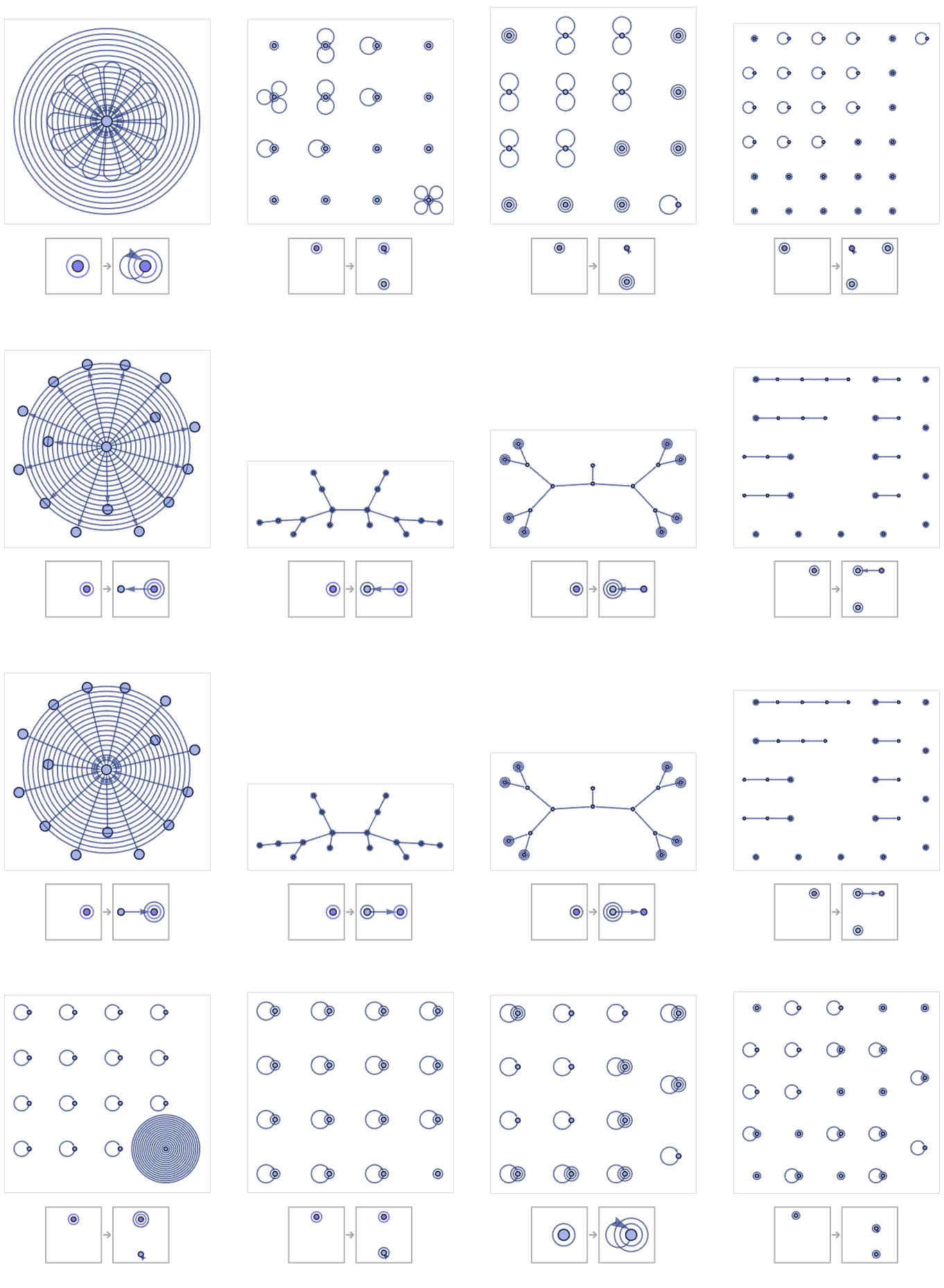
Many lead to disconnected hypergraphs; four lead to binary trees with structures we have already seen. ({{x}}→{{x,y},{x},{y}} is a 1₂  1₂2₁ rule that gives the same result as the very first 1₂  2₂ rule we saw.

Rules for a single unary relation can never give structures more complex than trees, though the morphology of the trees can become slightly more elaborate:

GraphicsGrid[ Transpose[{Show[ ResourceFunction["WolframModel"][#1, #2, #3, "FinalStatePlot"], ImageSize -> 180], RulePlot[ResourceFunction["WolframModel"][#1], ImageSize -> 180]} & @@@ {{{{x}} -> {{x, y}, {x}, {x}, {y}}, {{0}}, 4}, {{{x}} -> {{x, y}, {y}, {y}, {y}}, {{0}}, 5}, {{{x}} -> {{x, y, z}, {y}, {z}}, {{0}}, 7}}], Alignment -> {Automatic, {Bottom, Top}}, ImageSize -> 600]