5.14 Foliations and Coordinates on Causal Graphs

One way to describe a causal graph is to say that it defines the partial ordering of events in a system—or, in other words, it is a representation of a poset. (The actual graph is essentially the Hasse diagram of the poset (e.g. [69]).) Any particular sequence of updating events can then be thought of as a particular total ordering of the events.

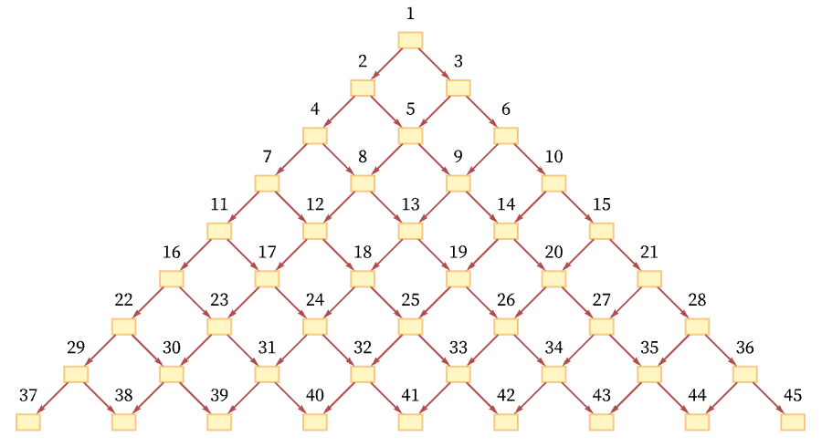
As a simple example, consider a grid causal graph (as generated, for example, by the rule BA  AB):

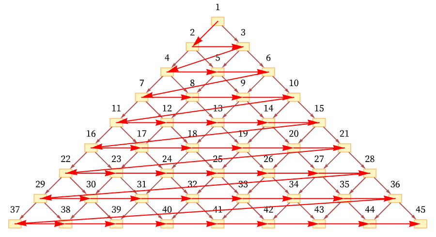
One total ordering of events consistent with all the causal relations in the graph is a “breadth-first scan” [70]:

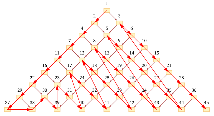
But another possible ordering is a “depth-first scan” [71]:

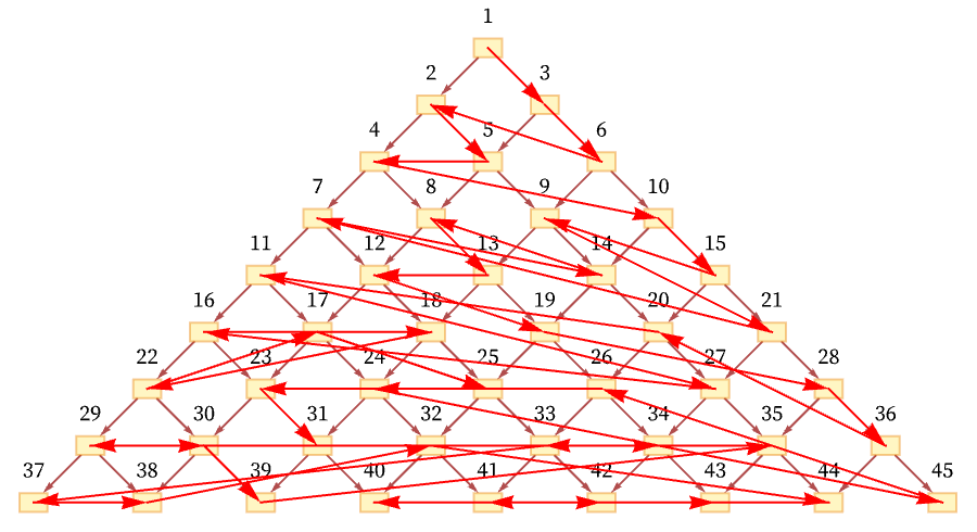
Another conceivable ordering would be:

And in general there are many orderings consistent with the relations defined by the causal graph. For the particular graph shown here, out of the n! conceivable orderings of nodes 1 through n, the orderings consistent with the causal relations correspond to possible Young tableaux, and the number of them is equal to the number of involutions (self-inverse permutations) of n elements (e.g. [11:A000085]) which is asymptotically a little larger than times n!.

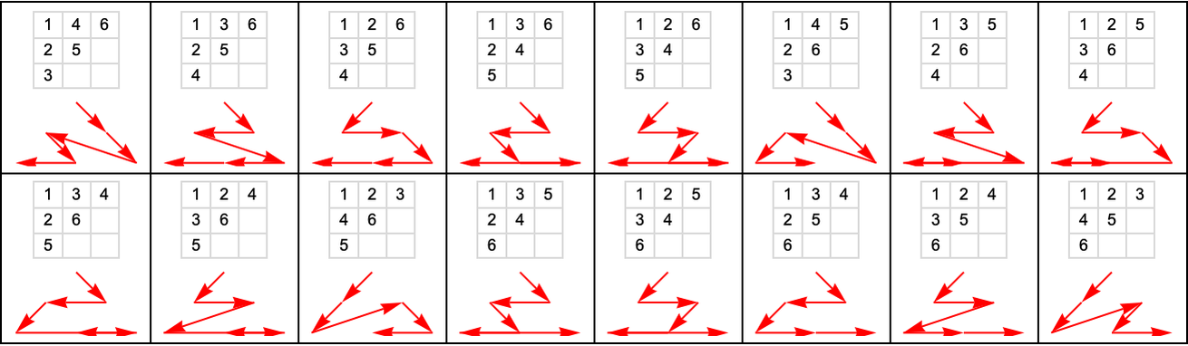
Here are the possible causal orderings that visit nodes 1 through 6 above (out of all 6! = 720 orderings):

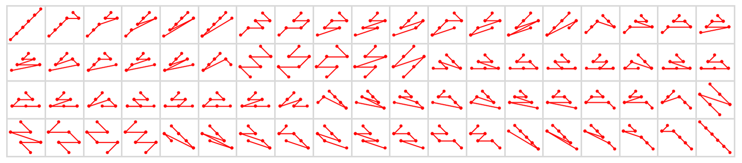
And here are all 76 possible causal orderings that visit any six nodes starting with node 1:

But while a great many total orderings are in principle possible, if one wants, for example, to think about large-scale limits, one usually wants to restrict oneself to orderings that can specified by (“reasonable”) foliations.

The idea of a foliation is to define a sequence of slices with the property that events on successive slices must occur in the order of the slices, but that events within a slice can occur in any order. So, for example, an immediate possible foliation of the causal graph above is just:

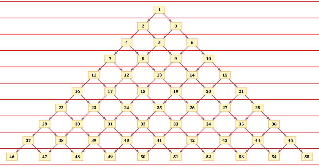
This foliation specifies that event 1 must happen first, but then events 2 and 3 can happen in any order, followed by events 4, 5 and 6 in any order, and so on.

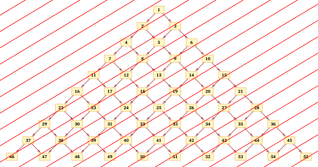
But another consistent foliation takes diagonal slices (with actual locations of events in the diagram being thought of as the centers of the boxes):

And so long as the diagonals are not steeper than the connections in the causal graph, this foliation will again lead to orderings that are consistent with the partial order defined by the causal graph. (For example, here event 1 must occur first, followed by event 2, followed by events 3 and 4 in any order, and so on.)

Particularly if the diagonals are steeper, multiple events will often happen in a single slice (as we see with events 4 and 7 here):

Now let us consider how this relates to taking the limit of a large number of events. If it were not for the directedness of the graph, we could do as we did in 4.17, and just imagine a process of refinement that leads to a manifold. But the Euclidean space that is the model for the manifold does not immediately have a way to capture the directedness of the graph, and so we need to do a little more.

But this is a place where foliations help. Because within a slice of a foliation we have events that can happen in any order. And at least for our string substitution system, the events can be thought of in the limit as being on a one-dimensional manifold, with a coordinate related to position on the string. And then there is just a second coordinate that is the index of the slices in the foliation.

But if the limit of our causal graph is a continuous space, we should be able to have a consistent notion of “distance between events”. For events that are “out of order”, the distance should be undefined (or perhaps infinite). But for other events, we should be able to compute the distance in terms of the coordinate (say t) that indexes the slices in the foliation and the coordinate (say x) within the slices.

Given the particular setup of diagonal slices on a causal graph that is a grid, there is a unique distance function that is independent of the angle of the slices, which can be expressed in terms of the coordinate differences Δt and Δx:

This function is exactly the standard Minkowski metric for a Lorentzian manifold [72][73], and we will encounter it again in section 8 when we discuss potential connections to physics. But here the metric is simply an abstract way to express distance in the limit of our causal graphs for string substitution systems.

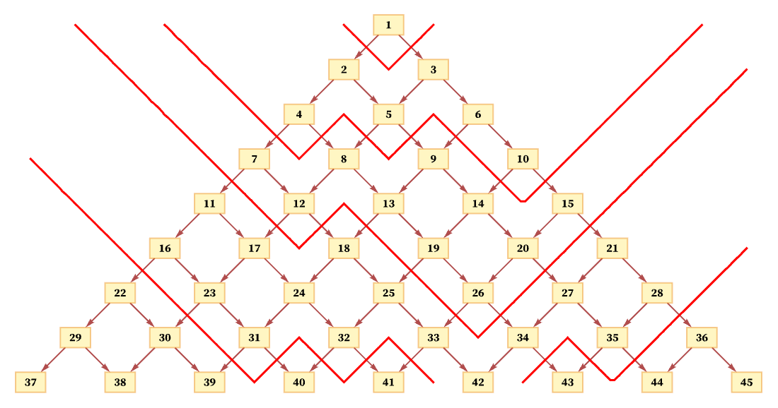
What happens if we use a different foliation? For example, a foliation like the following also leads to orderings of events that are consistent with the partial ordering required by the causal graph:

The process of limiting to a manifold is more complicated here. We can start by defining a “lapse function” α(t,x) (in analogy with the ADM formalism of general relativity [74][75]) which effectively says “how thick” each slice of the foliation is at each position. (If we also wanted to skew our foliations, we could include a “shift vector” as well.) And in the limit we can potentially define a distance by integrating along the shortest path from one point to another.

In a sense, however, even by imagining that there is a reasonable function α(t,x) that depends on real variables t and x we are implicitly assuming that our foliation has a certain simplicity and structure—and is not trying to reproduce some of the more circuitous total orderings at the beginning of this subsection.

But in a sense the question of what type of foliation we need to consider depends on what we want to use it for. And in making potential connections with physics, foliations will in effect be how we parametrize observers. And as soon as we assume that observers are limited in their computational capabilities, this puts constraints on the types of foliations we need to consider.