A Class of Models with the Potential to Represent Fundamental Physics
  1. Introduction
  2. Basic Form of Models
  3. Typical Behaviors
  4. Limiting Behavior and Emergent Geometry
  5. The Updating Process for String Substitution Systems
  6. The Updating Process in Our Models
  7. Equivalence and Computation in Our Models
  8. Potential Relation to Physics
  9. Additional Material
  10. References
  11. Index

6.9 Foliations of Causal Graphs

At least in a causal invariant system, the structure of the causal graph is always the same, and it defines the causal relationships that exist between updating events. But in relating the causal graph to actual underlying evolution histories for the system, we need to specify how we want to foliate the causal graphor, in effect, how we want to define “steps” in the evolution of the system.

As an example, consider the rule:

{{x, y}, {z, y}} -> {{x, z}, {y, z}, {w, z}}

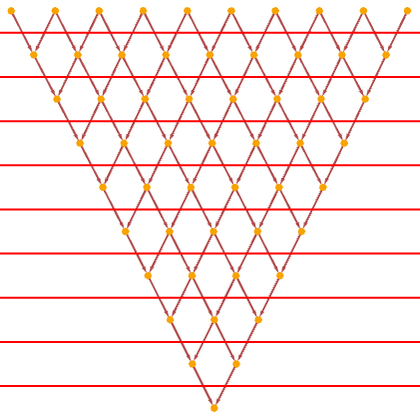
(This rule is probably not causal invariant, but this fact will not affect our discussion here.) The most obvious foliation for the causal graph basically follows our standard updating order:

CloudGet["https://wolfr.am/KXgcRNRJ"];evolution = ResourceFunction[ "WolframModel"][{{x, y}, {z, y}} -> {{x, z}, {y, z}, {w, z}}, {{0, 0}, {0, 0}}, 12]; gg = Graph[evolution["LayeredCausalGraph"]]; GraphPlot[gg, Epilog -> {Directive[Red], straightFoliationLines[{1/2, 0}, {0, 0}, (# &), {0, 1}]}]

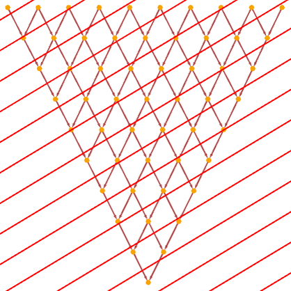
But this is not the only foliation we can use. In fact, we can divide the graph into slices in any way, so long as the slices respect the causal relationships defined by the graph, in the sense that within a slice the causal relationships allow the events to occur in any order, and between successive slices events must occur in the order of the slices. And with these criteria, for example, another possible foliation is:

CloudGet["https://wolfr.am/KXgcRNRJ"]; (*drawFoliation*) gg = Graph[ ResourceFunction[ "WolframModel"][ {{x, y}, {z, y}} -> {{x, z}, {y, z}, {w, z}}, {{0, 0}, {0, 0}}, 12, "LayeredCausalGraph"]]; semiRandomWMFoliation = {{1}, {1, 2, 4, 6, 9, 3}, {1, 2, 4, 6, 9, 3, 13, 19, 12, 26, 36, 5, 7, 10, 51, 14, 69, 18, 8, 25, 11, 34, 20, 35, 50, 17}, {1, 2, 4, 6, 9, 3, 13, 19, 12, 26, 36, 5, 7, 10, 51, 14, 69, 18, 8, 25, 11, 34, 20, 35, 50, 17, 24, 68, 47, 15, 92, 27, 48, 37, 21, 28, 42, 22, 30, 16, 32, 23, 33, 46, 64, 90, 94, 65, 88, 49, 67, 91, 66, 89}}; Quiet[drawFoliation[gg, semiRandomWMFoliation, Directive[Red]], FindRoot::cvmit]

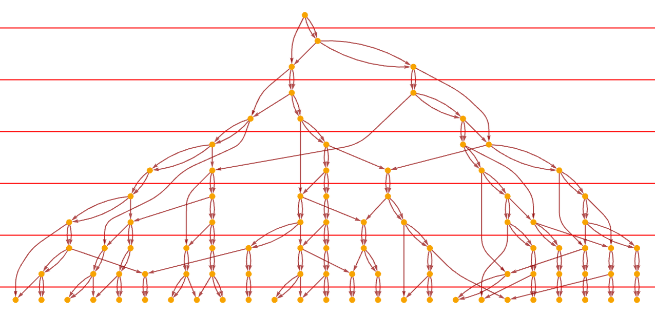
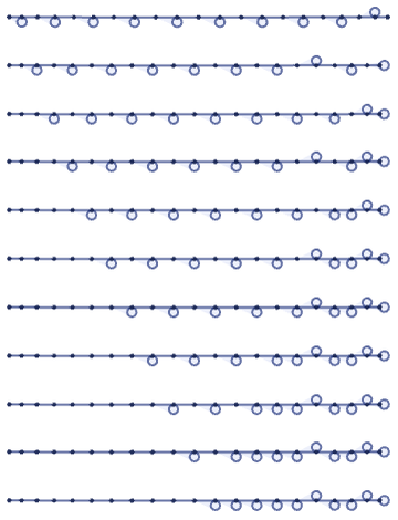
With the first foliation shown above, the hypergraphs from what we consider to be the first “few steps” in the evolution of the underlying rule are:

evolution = ResourceFunction[ "WolframModel"][{{x, y}, {z, y}} -> {{x, z}, {y, z}, {w, z}}, {{0, 0}, {0, 0}}, 12]; ResourceFunction["WolframModelPlot"][#, "MaxImageSize" -> 100] & /@ Join[{evolution[0]}, evolution["StatesList"][[2 ;; ;; 2]], {evolution["FinalState"]}]

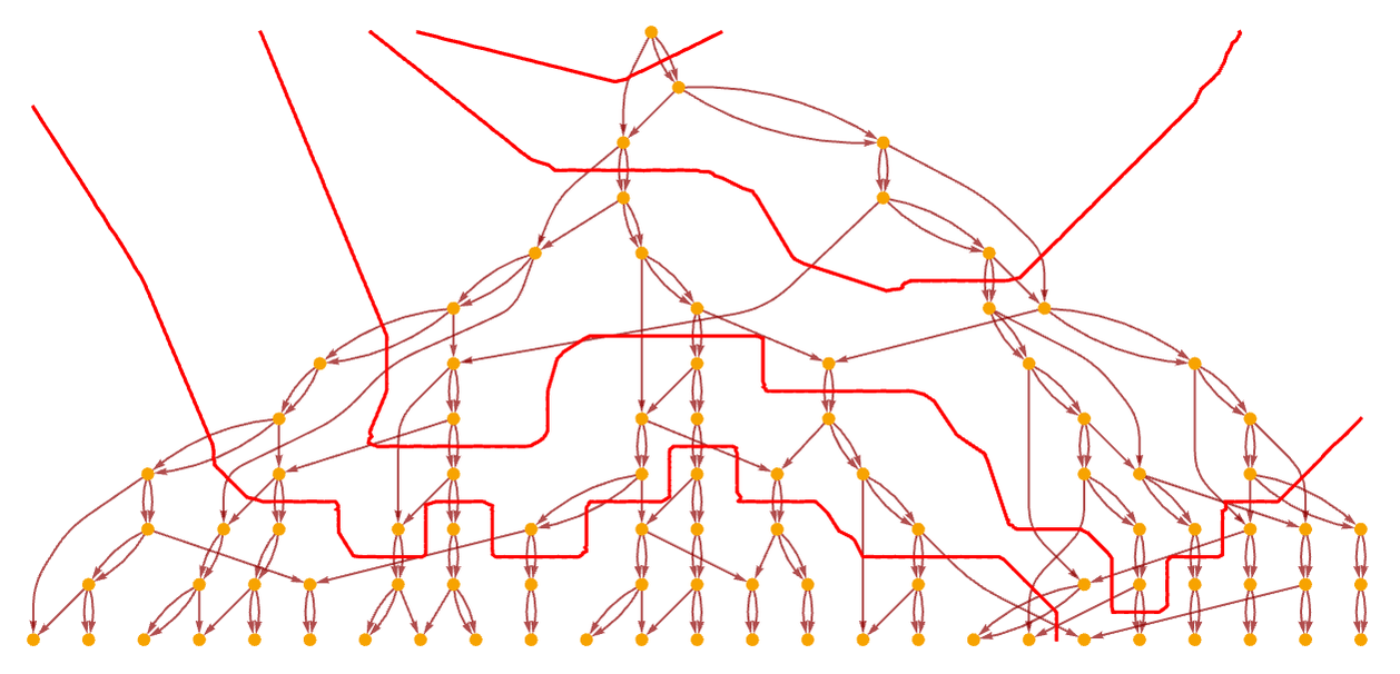
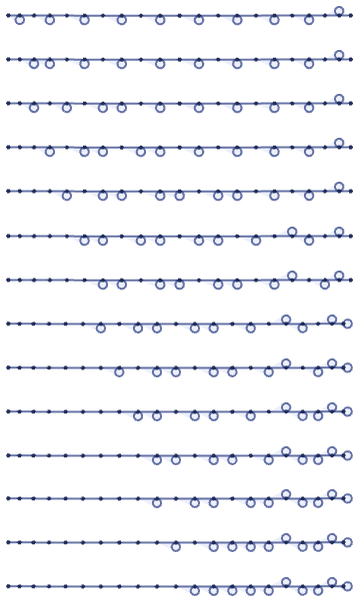
But the second foliation in effect has a different (and coarser) definition of “steps”, and with this foliation the first few steps would be:

evolution = ResourceFunction[ "WolframModel"][{{x, y}, {z, y}} -> {{x, z}, {y, z}, {w, z}}, {{0, 0}, {0, 0}}, 12]; semiRandomWMFoliation = {{1}, {1, 2, 4, 6, 9, 3}, {1, 2, 4, 6, 9, 3, 13, 19, 12, 26, 36, 5, 7, 10, 51, 14, 69, 18, 8, 25, 11, 34, 20, 35, 50, 17}, {1, 2, 4, 6, 9, 3, 13, 19, 12, 26, 36, 5, 7, 10, 51, 14, 69, 18, 8, 25, 11, 34, 20, 35, 50, 17, 24, 68, 47, 15, 92, 27, 48, 37, 21, 28, 42, 22, 30, 16, 32, 23, 33, 46, 64, 90, 94, 65, 88, 49, 67, 91, 66, 89}}; applyEvents[evolution_, events_] := evolution["AllEventsEdgesList"][[ Fold[Join[ DeleteCases[#, Alternatives @@ #2[[2, 1]]], #2[[2, 2]]] &, {}, evolution["EventsList", "IncludeBoundaryEvents" -> "Initial"][[ Join[{1}, events + 1]]]]]]; ResourceFunction["WolframModelPlot"][applyEvents[evolution, #], "MaxImageSize" -> 100] & /@ Join[{{}}, semiRandomWMFoliation, {Range[evolution["EventsCount"]]}]

When we discussed foliations in the context of string substitution systems, there were a number of simplifying features in our discussion. First, the underlying system fundamentally involved a linear string of elements. And second, the main causal graph we actually considered was a simple grid.

With a rule like

{{x, y, y}, {y, z}} -> {{x, y}, {y, z, z}}
RulePlot[ResourceFunction[ "WolframModel"][{{1, 2, 2}, {2, 3}} -> {{1, 2}, {2, 3, 3}}]]

we can also get a simple grid causal graph (and this rule happens to be causal invariant). With the obvious foliation

CloudGet["https://wolfr.am/KXgcRNRJ"];toState[str_] := MapThread[ If[# == "B", Append[#2, Last[#2]], #2] &, {Characters[str], Partition[Range[StringLength[str] + 1], 2, 1]}]; ResourceFunction[ "WolframModel"][{{1, 2, 2}, {2, 3}} -> {{1, 2}, {2, 3, 3}}, toState[StringJoin[Table["BA", 10]]], Infinity]["LayeredCausalGraph", Epilog -> straightFoliationLines[{1, 0}, {0, 0}]]

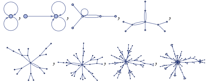
the steps in the evolution of the underlying system from a particular initial condition are:

toState[str_] := MapThread[ If[# == "B", Append[#2, Last[#2]], #2] &, {Characters[str], Partition[Range[StringLength[str] + 1], 2, 1]}]; ResourceFunction[ "WolframModel"][{{1, 2, 2}, {2, 3}} -> {{1, 2}, {2, 3, 3}}, toState[StringJoin[Table["BA", 10]]], Infinity, "StatesPlotsList"] // Column

But given the grid structure of the causal graph, we can use the same diagonal slice method for generating foliations that we did in 5.14. And for example with the foliation

CloudGet["https://wolfr.am/KXgcRNRJ"];toState[str_] := MapThread[ If[# == "B", Append[#2, Last[#2]], #2] &, {Characters[str], Partition[Range[StringLength[str] + 1], 2, 1]}]; ResourceFunction[ "WolframModel"][{{1, 2, 2}, {2, 3}} -> {{1, 2}, {2, 3, 3}}, toState[StringJoin[Table["BA", 10]]], Infinity]["LayeredCausalGraph", Epilog -> straightFoliationLines[{1, 0}, {0.6, 0}, # &, {-0.4, 0}]]

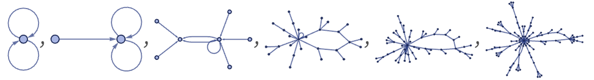
there are more steps involved in the evolution of the system:

sortingEvolution = ResourceFunction[ "WolframModel"][{{1, 2, 2}, {2, 3}} -> {{1, 2}, {2, 3, 3}}, toState[StringJoin[Table["BA", 10]]], Infinity]; toState[str_] := MapThread[ If[# == "B", Append[#2, Last[#2]], #2] &, {Characters[str], Partition[Range[StringLength[str] + 1], 2, 1]}]; applyEvents[evolution_, events_] := evolution["AllEventsEdgesList"][[ Fold[Join[ DeleteCases[#, Alternatives @@ #2[[2, 1]]], #2[[2, 2]]] &, {}, evolution["EventsList", "IncludeBoundaryEvents" -> "Initial"][[ Join[{1}, events + 1]]]]]]; ResourceFunction["WolframModelPlot"][ applyEvents[sortingEvolution, #]] & /@ FoldList[Join, {}, {{1}, {2, 3}, {4, 11, 12}, {5, 6, 13, 14, 20, 21}, {7, 8, 15, 22, 28}, {9, 16, 17, 23, 24, 29, 30, 35}, {10, 18, 19, 25, 26, 31, 36}, {27, 32, 33, 37, 38, 41, 42}, {34, 39, 40, 43, 46}, {44, 45, 47, 48, 50}, {49, 51}, {52, 53, 54}, {55}}] // Column

But when the causal graph does not have such a simple structure, the definition of foliations can be much more complicated. When the causal graph at least in some statistical sense limits to a sufficiently uniform structure, it should be possible to set up foliations that are analogous to the diagonal slices. And even in other cases, it will often be possible to set up foliations that can be described, for example, by the kind of lapse functions we discussed in 5.14.

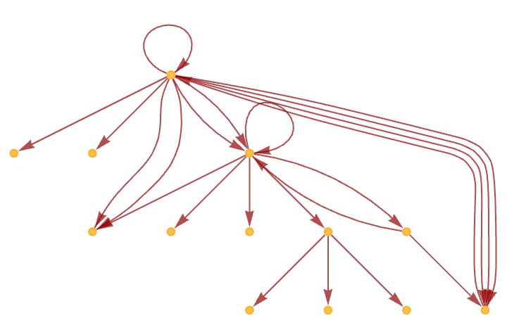
But there is one issue that can make it impossible to set up any reasonable “progressive” foliation of a causal graph at all, and that is the issue of loops. This issue is actually already present even in the case of string substitution systems (and even causal invariant ones). Consider for example the rule:

{"AA" -> "A", "A" -> "AA"}

Starting from AA the multiway causal graph for this rule is:

LayeredGraphPlot[ ResourceFunction["MultiwaySystem"][{"AA" -> "A", "A" -> "AA"}, "AA", 3, "CausalGraph"], AspectRatio -> 1/2]

But note here the presence of several loops. And looking at the states graph in this case

ResourceFunction["MultiwaySystem"][{"AA" -> "A", "A" -> "AA"}, "AA", 3, "StatesGraph"]

one can see where these loops come from: they are reflections of the fact that in the evolution of the system, there are states that can repeatand where in a sense a state can return to its past.

Whenever this happens, there is no way to make a progressive foliation in which events in future slices systematically depend only on events in earlier slices. (In the continuum limit, the analog is failure of strong hyperbolicity [86]; loops are the analog of closed timelike curves (e.g. [75])) (Self-loops also cause trouble for progressive foliations by forcing events to happen repeatedly within a slice, rather than only affecting later slices.)

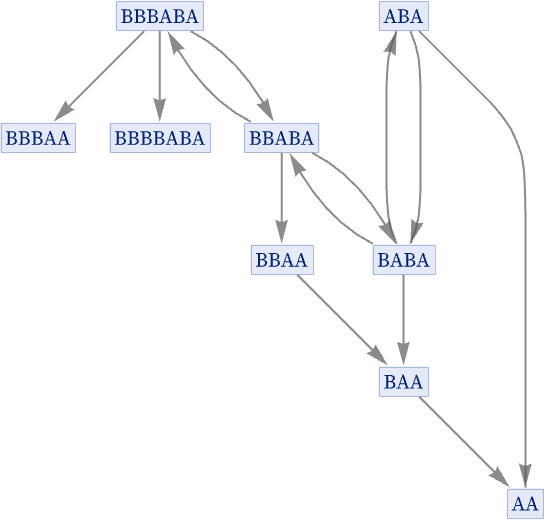
The phenomenon of loops is quite common in string substitution systems, and already happens with the trivial rule A A. It also happens for example with a rule like:

{"AB" -> "BAB", "BA" -> "A"}

Starting with ABA, this gives the causal graph

LayeredGraphPlot[ ResourceFunction["MultiwaySystem"][{"AB" -> "BAB", "BA" -> "A"}, "ABA", 4, "CausalGraphStructure"]]

and has a states graph:

Graph[ResourceFunction["MultiwaySystem"][{"AB" -> "BAB", "BA" -> "A"}, "ABA", 4, "StatesGraph"], GraphLayout -> {"LayeredDigraphEmbedding", "RootVertex" -> "ABA"}]

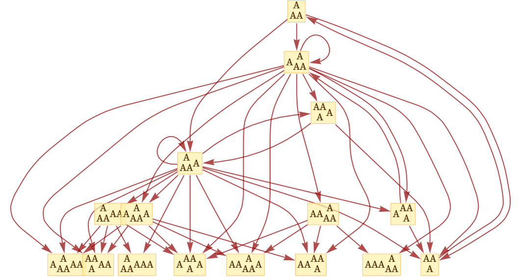
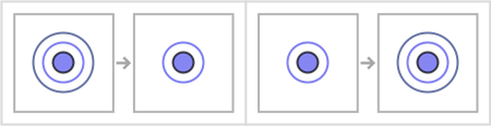
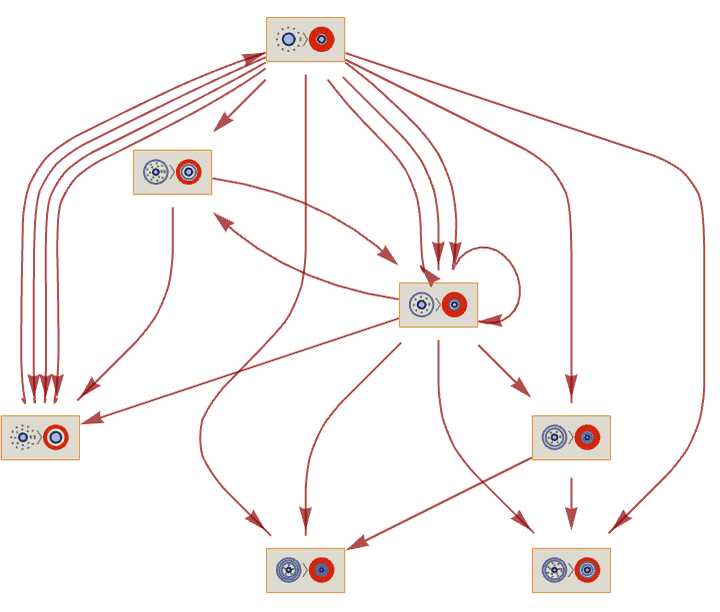
Loops can also happen in our models. Consider for example the very simple rule:

{{{x}, {x}} -> {{x}}, {{x}} -> {{x}, {x}}}
RulePlot[ResourceFunction[ "WolframModel"][{{{x}, {x}} -> {{x}}, {{x}} -> {{x}, {x}}}]]

The multiway graph for this rule is:

ResourceFunction["MultiwaySystem"][ "WolframModel" -> {{{0}, {0}} -> {{0}}, {{0}} -> {{0}, {0}}}, \ {{{0}}}, 3, "StatesGraph", VertexSize -> 1]

This contains loops, as does the corresponding causal graph:

Graph[ResourceFunction["MultiwaySystem"][ "WolframModel" -> {{{0}, {0}} -> {{0}}, {{0}} -> {{0}, {0}}}, \ {{{0}}}, 4, "CausalGraph"], VertexSize -> 1] // LayeredGraphPlot

(Note that the issue discussed in 6.1 of when we consider states “identical” as opposed to “equivalent” can again arise here. There are similar issues when we consider finite-size systems where the whole state inevitably repeatsand where in principle we can define a cyclic analog of our foliations.)