6.8 Large-Scale Structure of Causal Graphs

In section 5 we used the cone volume C_t to probe the large-scale structure of causal graphs generated by string substitution systems. Now we use C_t to probe the large-scale structure of causal graphs generated by our models.

Consider for example the rule

We found in section 4 that after a few steps, the volumes V_r of balls in the hypergraphs generated by this rule grow roughly like r^2.6, suggesting that in the limit the hypergraphs behave like a finite-dimensional space, with dimension ≈2.6.

The pictures below show the log differences in V_r and C_t for this rule after 15 steps of evolution:

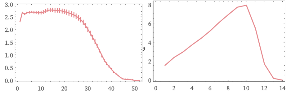
The linear increase in this plot implies exponential growth in C_t and indeed we find that for this rule:

This exponential growth—compared with the polynomial growth of V_r—implies that expansion according to this rule is in a sense sufficiently rapid that there is increasing causal disconnection between different parts of the system.

The other three 2₂  4₂ globular-hypergraph-generating rules shown in the previous subsection show similar exponential growth in C_t, at least over the number of steps of evolution tested.

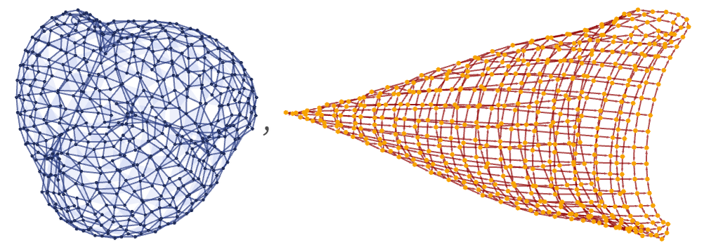
A rule such as

whose hypergraph and causal graph (after 500 steps) are respectively

gives the following for the log differences of V_r and C_t after 10,000 steps:

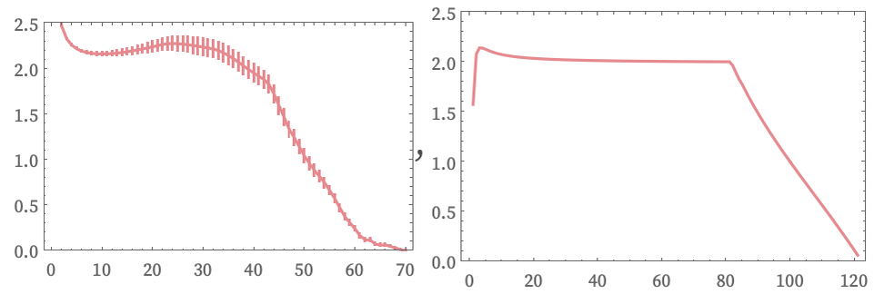
This implies that for this rule the hypergraphs it generates and its causal graph both effectively limit to finite-dimensional spaces, with the hypergraphs having dimension perhaps slightly over 2, and the causal graph having dimension 2.

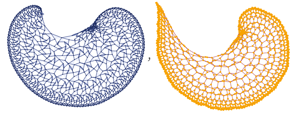
Consider now the rule:

The hypergraph and causal graph (after 1500 steps) for this rule are respectively:

The log differences of V_r and C_t after 10,000 steps are then:

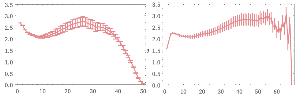
Both suggest limiting spaces with dimension 2, but with a certain amount of (negative) curvature.